Logistic Function

Calculates the logistic function value given parameters and input.

Usage

logist(x, x_0 = 0, L = 1, k = 1)

Arguments

x

Numeric vector, the values at which the logistic function will be evaluated.

x_0

Numeric, the x-value of the sigmoid's midpoint. Default is 0.

L

Numeric, the maximum value of the sigmoid. Default is 1.

k

Numeric, the steepness or slope of the sigmoid. Default is 1.

Value

A numeric vector of logistic function values.

Examples

x_vals <- seq(0, 10, by = 0.1)

# Calculate the features for each scenario
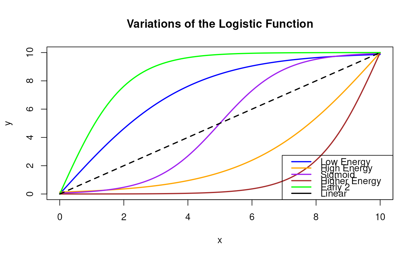
features_low_energy <- logist(x_vals, x_0 = 0, L = 2, k = 0.5) - 1
features_high_energy <- logist(x_vals, x_0 = 10, L = 2, k = 0.5)
features_sigmoid <- logist(x_vals - 5, x_0 = 0, L = 1, k = 1)
features_higher_energy <- logist(x_vals, x_0 = 10, L = 2, k = 1)
features_early2 <- logist(x_vals, x_0 = 0, L = 2, k = 1) - 1

# Base plot setup
plot(x_vals, features_low_energy * 10,
    type = "l", col = "blue",
    main = "Variations of the Logistic Function",
    xlab = "x", ylab = "y", ylim = c(0, 10), lwd = 2
)

# Adding other variations
lines(x_vals, features_high_energy * 10, col = "orange", lwd = 2)
lines(x_vals, features_sigmoid * 10, col = "purple", lwd = 2)
lines(x_vals, features_higher_energy * 10, col = "brown", lwd = 2)
lines(x_vals, features_early2 * 10, col = "green", lwd = 2)
lines(x_vals, x_vals, col = "black", lwd = 2, lty = 2)

legend("bottomright",
    legend = c("Low Energy", "High Energy", "Sigmoid", "Higher Energy", "Early 2", "Linear"),
    col = c("blue", "orange", "purple", "brown", "green", "black"),
    lty = 1,
    lwd = 2
)