2 Methylation trends in EB days 0-6
2.0.2 Load data
Load the data of methylation day 0-4:
## [1] 132052 24## [1] "d0_3a" "d0S_3a" "d1_3a" "d2_3a" "d3_3a" "d4_3a" "d0_3b"
## [8] "d0S_3b" "d1_3b" "d2_3b" "d3_3b" "d4_3b" "d0_tko" "d0S_tko"
## [15] "d1_tko" "d2_tko" "d3_tko" "d4_tko" "d0_wt" "d0S_wt" "d1_wt"
## [22] "d2_wt" "d3_wt" "d4_wt"2.0.3 Cluster
##  [1] "d0_3a"   "d0S_3a"  "d1_3a"   "d2_3a"   "d3_3a"   "d4_3a"   "d0_3b"
##  [8] "d0S_3b"  "d1_3b"   "d2_3b"   "d3_3b"   "d4_3b"   "d0_tko"  "d0S_tko"
## [15] "d1_tko"  "d2_tko"  "d3_tko"  "d4_tko"  "d0_wt"   "d0S_wt"  "d1_wt"
## [22] "d2_wt" "d3_wt" "d4_wt"m_column_order <- c(
"d0_3a", "d1_3a", "d2_3a", "d3_3a", "d4_3a",
"d0_3b", "d1_3b", "d2_3b", "d3_3b", "d4_3b",
"d0_wt", "d1_wt", "d2_wt", "d3_wt", "d4_wt",
"d0_tko", "d1_tko", "d2_tko", "d3_tko", "d4_tko",
"d0S_3a", "d0S_3b", "d0S_wt", "d0S_tko"
)
m <- m[, m_column_order]
colnames(m)## [1] "d0_3a" "d1_3a" "d2_3a" "d3_3a" "d4_3a" "d0_3b" "d1_3b"
## [8] "d2_3b" "d3_3b" "d4_3b" "d0_wt" "d1_wt" "d2_wt" "d3_wt"
## [15] "d4_wt" "d0_tko" "d1_tko" "d2_tko" "d3_tko" "d4_tko" "d0S_3a"
## [22] "d0S_3b" "d0S_wt" "d0S_tko"K <- 60
km <- tglkmeans::TGL_kmeans(m, K, id_column=FALSE, seed=19) %cache_rds% here("output/meth_capt_clust.rds")## # A tibble: 10 x 2
## name value
## 1 1 1179
## 2 9 5459
## 3 19 2023
## 4 24 1573
## 5 30 1295
## 6 32 2810
## # ... with 4 more rowskm_m_3a <- rowSums(km$centers[,c("d1_3a","d2_3a","d3_3a","d4_3a")])
km_m_3b <- rowSums(km$centers[,c("d1_3b","d2_3b","d3_3b","d4_3b")])
km_m_wt <- rowSums(km$centers[,c("d1_wt","d2_wt","d3_wt","d4_wt")])
cent_dlt <- km$centers[,c("d1_3a","d2_3a","d3_3a","d4_3a")]-
km$centers[,c("d1_3b","d2_3b","d3_3b","d4_3b")]dlt24 <- cent_dlt[,2]-cent_dlt[,4]
clst_mod <- rep(0, K)
clst_mod[(km_m_3a-km_m_3b) < -0.3 & dlt24 > -0.05] <- 3
clst_mod[(km_m_3a-km_m_3b) < -0.2 & dlt24 < -0.05] <- 2
clst_mod[(km_m_3a-km_m_3b) > 0.2] <- 1smooth_n = floor(nrow(m)/1000)+1
km_mean_e = rowSums(km$centers)
tot_cent_dlt = rowSums(cent_dlt)
k_ord = order(ifelse(clst_mod==0,
km_mean_e,
abs(tot_cent_dlt)) + clst_mod*20)
clst_map <- 1:K
names(clst_map) <- as.character(k_ord)
clst <- km$cluster
clst_sorted <- clst_map[as.character(clst)]
km$cluster <- clst_sorted
km$centers <- km$centers[k_ord,]
rownames(km$centers) <- 1:K
m_ord <- order(km$cluster)m_s5 = apply(m[m_ord,-1],2, zoo::rollmean, smooth_n, fill=c('extend',NA,'extend'), na.rm=T)
colnames(m_s5) = colnames(m)[-1]## [1] 132052 23options(repr.plot.width = 8, repr.plot.height = 20)
plot_clust <- function() {
shades <- colorRampPalette(c("white", "#635547", "#DABE99","#C594BF","#B51D8D","darkred", "yellow"))(1000)
image(t(as.matrix(m_s5)),col=shades, xaxt='n', yaxt='n');
N = length(m_ord)
m_y = tapply((1:N)/N, km$cluster[m_ord], mean)
mtext(1:K, at = m_y, las=2, side= 2)
mtext(1:K, at = m_y, las=2, side= 4)
abline(h=tapply((1:N)/N, km$cluster[m_ord], max))
}
plot_clust()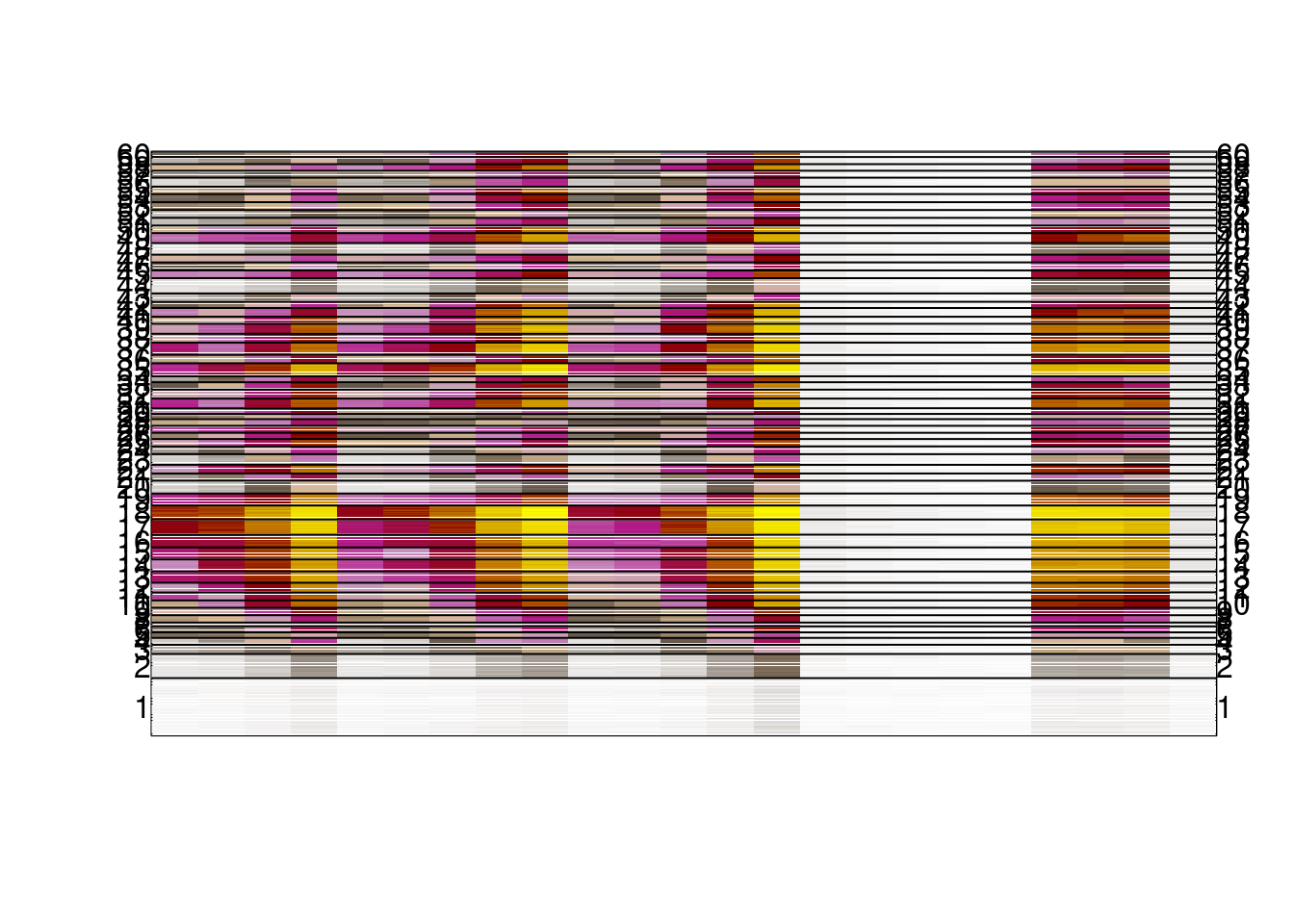
options(repr.plot.width = 3, repr.plot.height = 10)
plot_delta <- function(){
    delta = m_s5[,c("d1_3a","d2_3a","d3_3a","d4_3a")]-
            m_s5[,c("d1_3b","d2_3b","d3_3b","d4_3b")]

    dshades <- colorRampPalette(c("red","darkred","white","darkblue","blue"))(1000)
    image(pmin(pmax(t(as.matrix(delta)),-0.3),0.3),col=dshades,zlim=c(-0.3,0.3))
}
plot_delta()
2.0.4 Project DNMT1 data
all_clust_data <- calc_eb_cpg_meth(from = 0, to = 5, min_cov = 10, max_na = NULL, intervals = clust_intervs, iterator = clust_intervs, cache_fn = here("output/all_clust_data.tsv"), rm_meth_cov = TRUE)## [1] "chrom" "start" "end" "d0_d13ako" "d3_d13ako" "d4_d13ako"
## [7] "d0_d13bko" "d3_d13bko" "d4_d13bko" "d5_dko" "d0_ko1" "d0S_ko1"
## [13] "d1_ko1" "d2_ko1" "d3_ko1" "d4_ko1" "d5_ko1" "d0_3a"
## [19] "d0S_3a" "d1_3a" "d2_3a" "d3_3a" "d4_3a" "d5_3a"
## [25] "d0_3b" "d0S_3b" "d1_3b" "d2_3b" "d3_3b" "d4_3b"
## [31] "d5_3b" "d0_tko" "d0S_tko" "d1_tko" "d2_tko" "d3_tko"
## [37] "d4_tko" "d0_wt" "d0S_wt" "d1_wt" "d2_wt" "d3_wt"
## [43] "d4_wt" "d5_wt"m_column_order <- c(
"d0_3a", "d1_3a", "d2_3a", "d3_3a", "d4_3a",
"d0_3b", "d1_3b", "d2_3b", "d3_3b", "d4_3b",
"d0_wt", "d1_wt", "d2_wt", "d3_wt", "d4_wt",
"d0_tko", "d1_tko", "d2_tko", "d3_tko", "d4_tko",
"d0S_3a", "d0S_3b", "d0S_wt", "d0S_tko", "d0S_ko1",
"d0_ko1", "d1_ko1", "d2_ko1", "d3_ko1", "d4_ko1",
"d0_d13ako", "d3_d13ako", "d4_d13ako",
"d0_d13bko", "d3_d13bko", "d4_d13bko"
)
setdiff(colnames(all_clust_data)[-1:-3], m_column_order)## [1] "d5_dko" "d5_ko1" "d5_3a" "d5_3b" "d5_wt"## [1] "d0_3a" "d1_3a" "d2_3a" "d3_3a" "d4_3a" "d0_3b"
## [7] "d1_3b" "d2_3b" "d3_3b" "d4_3b" "d0_wt" "d1_wt"
## [13] "d2_wt" "d3_wt" "d4_wt" "d0_tko" "d1_tko" "d2_tko"
## [19] "d3_tko" "d4_tko" "d0S_3a" "d0S_3b" "d0S_wt" "d0S_tko"
## [25] "d0S_ko1" "d0_ko1" "d1_ko1" "d2_ko1" "d3_ko1" "d4_ko1"
## [31] "d0_d13ako" "d3_d13ako" "d4_d13ako" "d0_d13bko" "d3_d13bko" "d4_d13bko"## d0_3a d1_3a d2_3a d3_3a d4_3a d0_3b
## [1,] 0.01001037 0.01079793 0.004898041 0.01102023 0.01277668 0.005717633
## [2,] 0.01001037 0.01079793 0.004898041 0.01102023 0.01277668 0.005717633
## [3,] 0.01001037 0.01079793 0.004898041 0.01102023 0.01277668 0.005717633
## [4,] 0.01001037 0.01079793 0.004898041 0.01102023 0.01277668 0.005717633
## [5,] 0.01001037 0.01079793 0.004898041 0.01102023 0.01277668 0.005717633
## [6,] 0.01001037 0.01079793 0.004898041 0.01102023 0.01277668 0.005717633
## d1_3b d2_3b d3_3b d4_3b d0_wt d1_wt
## [1,] 0.007146658 0.008921023 0.01298582 0.01649393 0.006180905 0.006556652
## [2,] 0.007146658 0.008921023 0.01298582 0.01649393 0.006180905 0.006556652
## [3,] 0.007146658 0.008921023 0.01298582 0.01649393 0.006180905 0.006556652
## [4,] 0.007146658 0.008921023 0.01298582 0.01649393 0.006180905 0.006556652
## [5,] 0.007146658 0.008921023 0.01298582 0.01649393 0.006180905 0.006556652
## [6,] 0.007146658 0.008921023 0.01298582 0.01649393 0.006180905 0.006556652
## d2_wt d3_wt d4_wt d0_tko d1_tko d2_tko
## [1,] 0.01132803 0.01854894 0.02603882 0.005965149 0.004823037 0.004019872
## [2,] 0.01132803 0.01854894 0.02603882 0.005965149 0.004823037 0.004019872
## [3,] 0.01132803 0.01854894 0.02603882 0.005965149 0.004823037 0.004019872
## [4,] 0.01132803 0.01854894 0.02603882 0.005965149 0.004823037 0.004019872
## [5,] 0.01132803 0.01854894 0.02603882 0.005965149 0.004823037 0.004019872
## [6,] 0.01132803 0.01854894 0.02603882 0.005965149 0.004823037 0.004019872
## d3_tko d4_tko d0S_3a d0S_3b d0S_wt d0S_tko
## [1,] 0.005696785 0.006240729 0.01627394 0.01726621 0.02124627 0.007268556
## [2,] 0.005696785 0.006240729 0.01627394 0.01726621 0.02124627 0.007268556
## [3,] 0.005696785 0.006240729 0.01627394 0.01726621 0.02124627 0.007268556
## [4,] 0.005696785 0.006240729 0.01627394 0.01726621 0.02124627 0.007268556
## [5,] 0.005696785 0.006240729 0.01627394 0.01726621 0.02124627 0.007268556
## [6,] 0.005696785 0.006240729 0.01627394 0.01726621 0.02124627 0.007268556
## d0S_ko1 d0_ko1 d1_ko1 d2_ko1 d3_ko1 d4_ko1
## [1,] 0.01001541 0.004047823 0.006723765 0.007574284 0.01410948 0.007942855
## [2,] 0.01001541 0.004047823 0.006723765 0.007574284 0.01410948 0.007942855
## [3,] 0.01001541 0.004047823 0.006723765 0.007574284 0.01410948 0.007942855
## [4,] 0.01001541 0.004047823 0.006723765 0.007574284 0.01410948 0.007942855
## [5,] 0.01001541 0.004047823 0.006723765 0.007574284 0.01410948 0.007942855
## [6,] 0.01001541 0.004047823 0.006723765 0.007574284 0.01410948 0.007942855
## d0_d13ako d3_d13ako d4_d13ako d0_d13bko d3_d13bko d4_d13bko
## [1,] 0.008525676 0.0166642 0.01150588 0.006178614 0.01029716 0.005339577
## [2,] 0.008525676 0.0166642 0.01150588 0.006178614 0.01029716 0.005339577
## [3,] 0.008525676 0.0166642 0.01150588 0.006178614 0.01029716 0.005339577
## [4,] 0.008525676 0.0166642 0.01150588 0.006178614 0.01029716 0.005339577
## [5,] 0.008525676 0.0166642 0.01150588 0.006178614 0.01029716 0.005339577
## [6,] 0.008525676 0.0166642 0.01150588 0.006178614 0.01029716 0.005339577days <- strsplit(colnames(m_all_s5), split = "_") %>% map_chr(~ .x[1]) %>% gsub("d", "", .)
days[grep("0S", days)] <- c("A", "B", "WT", "TKO", "KO1")options(repr.plot.width = 20, repr.plot.height = 20)
shades <- colorRampPalette(c("white", "#635547", "#DABE99","#C594BF","#B51D8D","darkred", "yellow"))(1000)
image(t(as.matrix(m_all_s5)),col=shades, xaxt='n', yaxt='n');
N = length(m_ord)
m_y = tapply((1:N)/N, km$cluster[m_ord], mean)
mtext(1:K, at = m_y, las=2, side= 2)
mtext(1:K, at = m_y, las=2, side= 4)
axis(3, at = seq(0, 1, length = ncol(m_all_s5)), labels = days)
abline(h=tapply((1:N)/N, km$cluster[m_ord], max))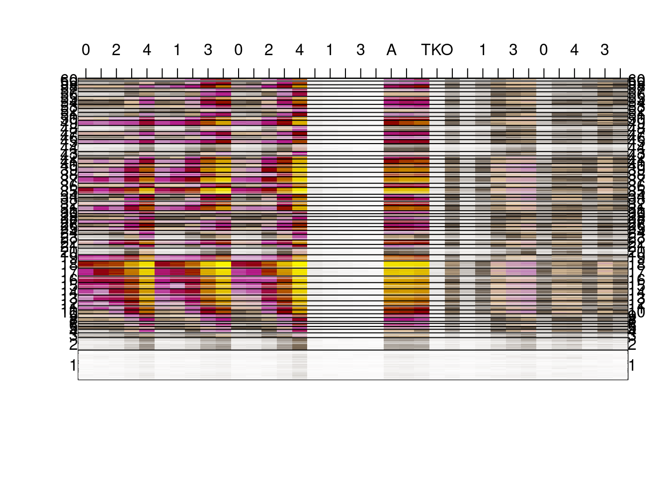
options(repr.plot.width = 3, repr.plot.height = 20)
delta = m_s5[,c("d1_3a","d2_3a","d3_3a","d4_3a")]-
m_s5[,c("d1_3b","d2_3b","d3_3b","d4_3b")]
dshades <- colorRampPalette(c("red","darkred","white","darkblue","blue"))(1000)
image(pmin(pmax(t(as.matrix(delta)),-0.3),0.3),col=dshades,zlim=c(-0.3,0.3))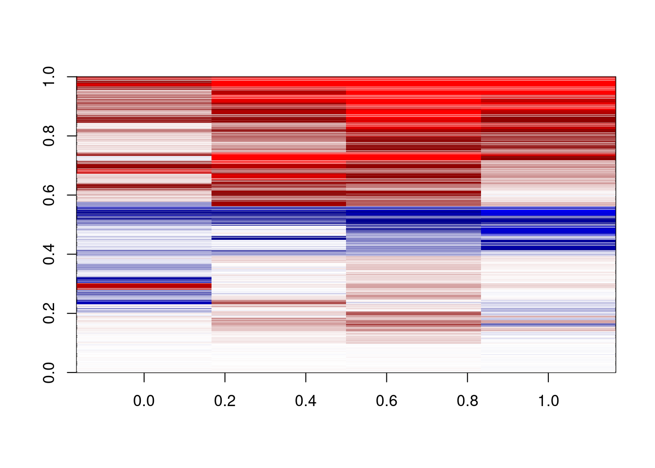
2.0.4.1 Trajectory per cluster
line_colors <- c("wt" = "darkblue", "3a" = "purple", "3b" = "orange", "tko" = "darkgray", "ko1" = "darkgreen", "d13ako" = "turquoise4", "d13bko" = "orangered4")df <- all_clust_data %>%
mutate(clust = km$cluster) %>%
group_by(clust) %>%
summarise_at(vars(starts_with("d")), mean, na.rm=TRUE) %>%
gather("samp", "meth", -clust) %>%
separate(samp, c("day", "line"), sep="_") %>%
filter(day != "d0S", day != "d5") %>%
mutate(day = gsub("d", "", day)) %>%
mutate(line = factor(line, levels = names(line_colors)))options(repr.plot.width = 5, repr.plot.height = 15)
df %>%
filter(clust %in% chosen_clusters) %>%
mutate(clust = factor(clust), clust = forcats::fct_rev(clust)) %>%
ggplot(aes(x=day, y=meth, color=line, group=line)) +
geom_line() +
geom_point(size=0.5) +
xlab("EB day") +
ylab("Meth.") +
theme(aspect.ratio = 1) +
facet_grid(clust~.) +
scale_color_manual(name = "", values = line_colors) +
scale_y_continuous(limits=c(0,1))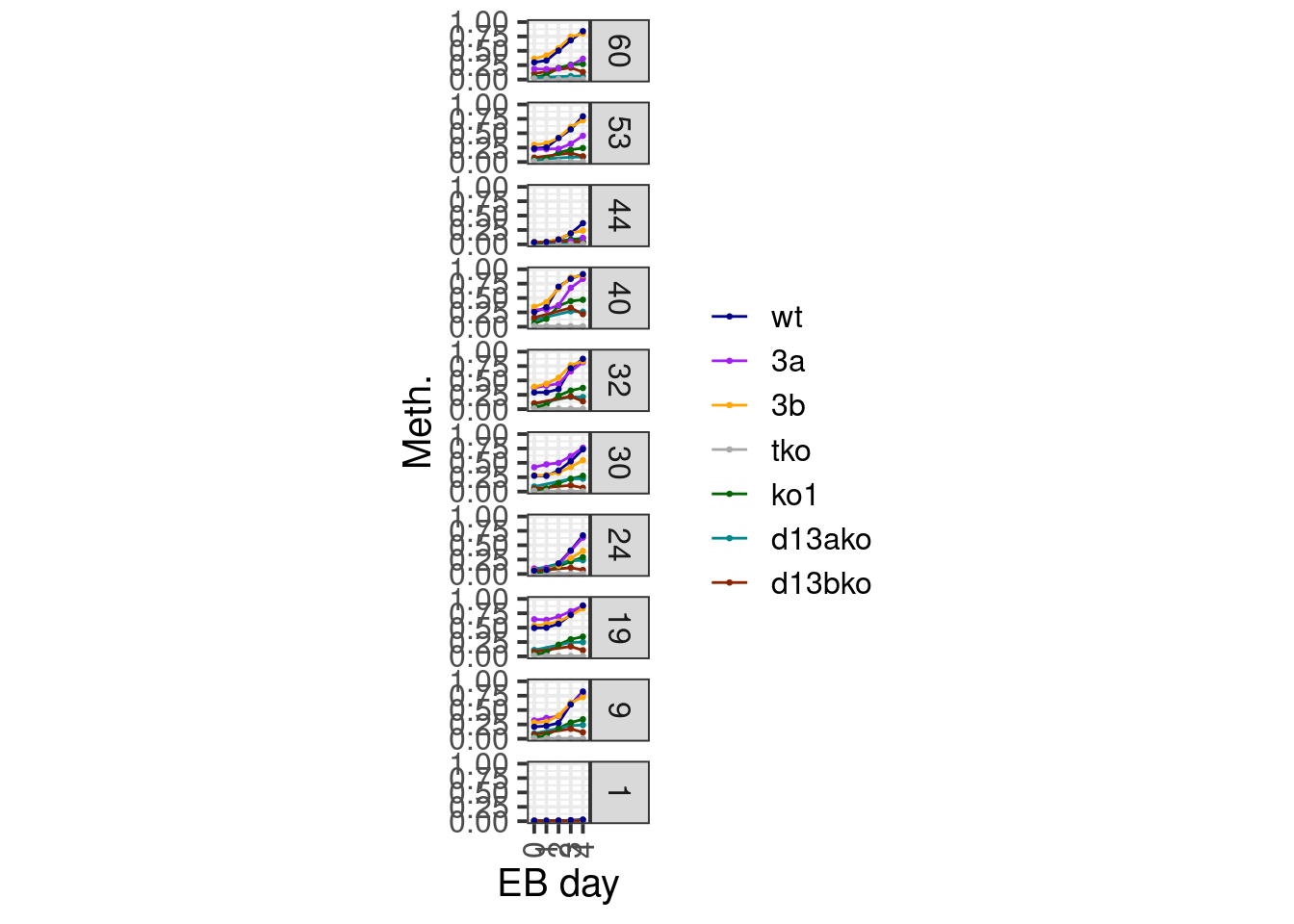
2.1 Plot global EB trends
2.1.1 Figure 4A
cpg_meth1 <- gextract.left_join("seq.CG_500_mean", intervals=cpg_meth, iterator=cpg_meth, colnames="cg_cont") %>% select(-(chrom1:end1)) %>% select(chrom, start, end, cg_cont, everything()) %>% as_tibble()line_colors <- c("wt" = "darkblue", "3a" = "purple", "3b" = "orange", "tko" = "darkgray")
df <- cpg_meth1 %>%
mutate(cg_cont = cut(cg_cont, c(0,0.03,0.08,0.15), include.lowest=TRUE, labels=c("low", "mid", "high"))) %>%
group_by(cg_cont) %>%
summarise_at(vars(starts_with("d")), mean, na.rm=TRUE) %>%
gather("samp", "meth", -cg_cont) %>%
separate(samp, c("day", "line"), sep="_") %>%
filter(day != "d0S") %>%
mutate(day = gsub("d", "", day)) %>%
mutate(line = factor(line, levels = names(line_colors)))options(repr.plot.width = 14, repr.plot.height = 7)
p_high <- df %>% filter(cg_cont == "high") %>% ggplot(aes(x=day, y=meth, color=line, group=line)) + geom_line() + geom_point(size=0.5) + ggtitle("High CpG content") + xlab("EB day") + ylab("Meth.") + theme(aspect.ratio = 1) + scale_color_manual(name = "", values = line_colors) + scale_y_continuous(limits=c(0,0.8))
p_low <- df %>% filter(cg_cont == "low") %>% ggplot(aes(x=day, y=meth, color=line, group=line)) + geom_line() + geom_point(size=0.5) + ggtitle("Low CpG content") + xlab("EB day") + ylab("Meth.") + theme(aspect.ratio = 1) + scale_color_manual(name = "", values = line_colors) + scale_y_continuous(limits=c(0,0.8))
p_high + p_low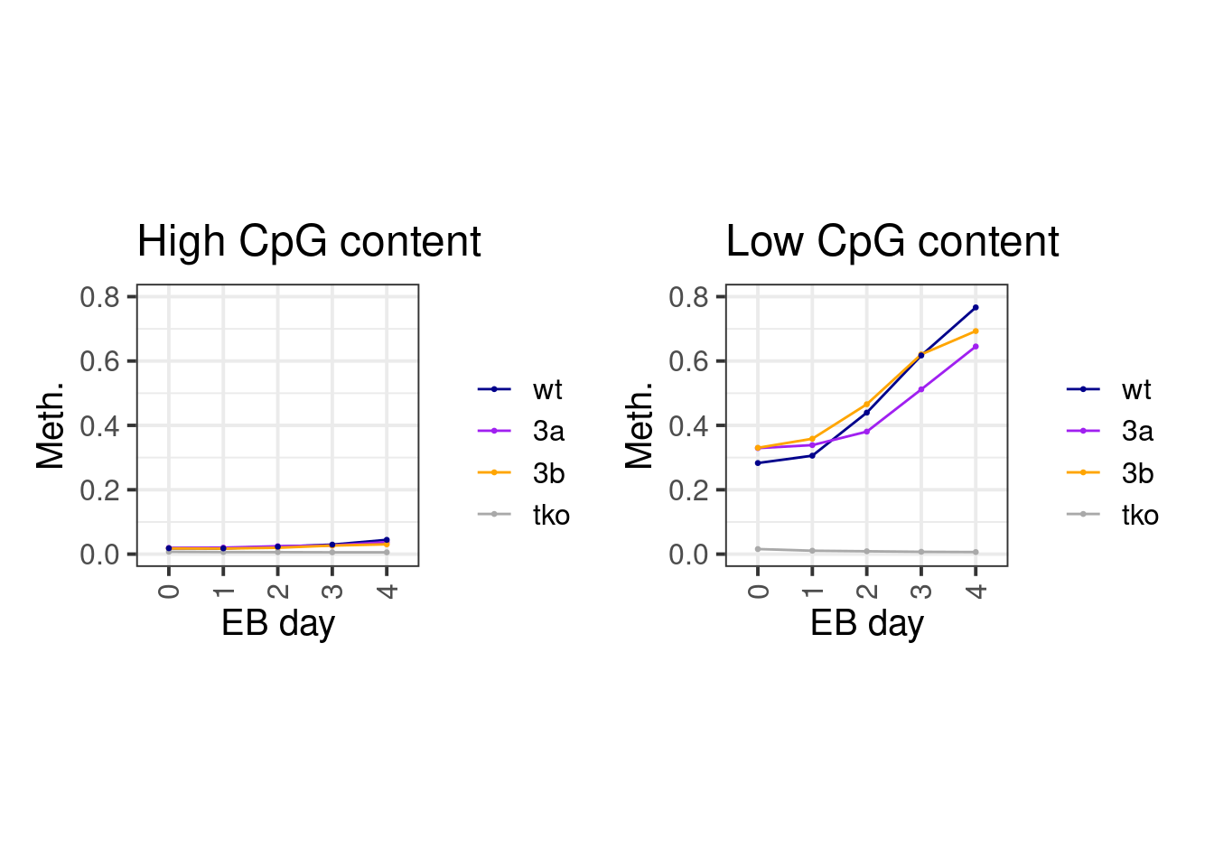
2.1.2 Extended Data Figure 8K
Same for X chromosome
line_colors <- c("wt" = "darkblue", "3a" = "purple", "3b" = "orange", "tko" = "darkgray")
df <- cpg_meth1 %>%
mutate(type = case_when(chrom == "chrX" ~ "X", TRUE ~ "autosome")) %>%
mutate(cg_cont = cut(cg_cont, c(0,0.03,0.08,0.15), include.lowest=TRUE, labels=c("low", "mid", "high"))) %>%
group_by(type, cg_cont) %>%
summarise_at(vars(starts_with("d")), mean, na.rm=TRUE) %>%
gather("samp", "meth", -cg_cont, -type) %>%
separate(samp, c("day", "line"), sep="_") %>%
filter(day != "d0S") %>%
mutate(day = gsub("d", "", day)) %>%
mutate(line = factor(line, levels = names(line_colors)))options(repr.plot.width = 14, repr.plot.height = 7)
p_high_x <- df %>% filter(type == "X", cg_cont == "high") %>% ggplot(aes(x=day, y=meth, color=line, group=line)) + geom_line() + geom_point(size=0.5) + ggtitle("X chromosome:\nHigh CpG content") + xlab("EB day") + ylab("Meth.") + theme(aspect.ratio = 1) + scale_color_manual(name = "", values = line_colors) + scale_y_continuous(limits=c(0,0.8))
p_low_x <- df %>% filter(type == "X", cg_cont == "low") %>% ggplot(aes(x=day, y=meth, color=line, group=line)) + geom_line() + geom_point(size=0.5) + ggtitle("X chromosome:\nLow CpG content") + xlab("EB day") + ylab("Meth.") + theme(aspect.ratio = 1) + scale_color_manual(name = "", values = line_colors) + scale_y_continuous(limits=c(0,0.8))
p_high_x + p_low_x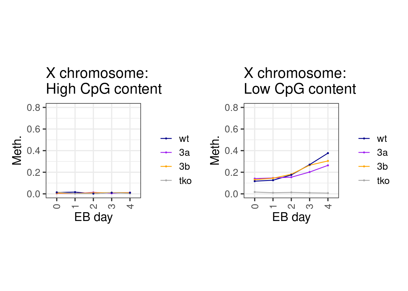
2.2 cluster methylation in days 5 and 6 with DKO
2.2.1 Project DKO on day 1-4 clusters
all_clust_data <- calc_eb_cpg_meth(from = 0, to = 6, min_cov = 10, max_na = NULL, intervals = clust_intervs, iterator = clust_intervs, cache_fn = here("output/all_clust_data_day1_to_6.tsv"), rm_meth_cov = TRUE, tracks_key = NULL)m_column_order <- c(
"d0_3a", "d1_3a", "d2_3a", "d3_3a", "d4_3a", "d5_3a", "d6_3a",
"d0_3b", "d1_3b", "d2_3b", "d3_3b", "d4_3b", "d5_3b", "d6_3b",
"d0_wt", "d1_wt", "d2_wt", "d3_wt", "d4_wt", "d5_wt", "d6_wt",
"d5_dko", "d6_dko",
"d0_tko", "d1_tko", "d2_tko", "d3_tko", "d4_tko",
"d0S_3a", "d0S_3b", "d0S_wt", "d0S_tko"
)
setdiff(colnames(all_clust_data)[-1:-3], m_column_order)## [1] "d0_d13ako" "d3_d13ako" "d4_d13ako" "d0_d13bko" "d3_d13bko" "d4_d13bko"
## [7] "d0_ko1" "d0S_ko1" "d1_ko1" "d2_ko1" "d3_ko1" "d4_ko1"
## [13] "d5_ko1"## character(0)## [1] "d0_3a" "d1_3a" "d2_3a" "d3_3a" "d4_3a" "d5_3a" "d6_3a"
## [8] "d0_3b" "d1_3b" "d2_3b" "d3_3b" "d4_3b" "d5_3b" "d6_3b"
## [15] "d0_wt" "d1_wt" "d2_wt" "d3_wt" "d4_wt" "d5_wt" "d6_wt"
## [22] "d5_dko" "d6_dko" "d0_tko" "d1_tko" "d2_tko" "d3_tko" "d4_tko"
## [29] "d0S_3a" "d0S_3b" "d0S_wt" "d0S_tko"## d0_3a d1_3a d2_3a d3_3a d4_3a d5_3a d6_3a
## [1,] 0.01001037 0.01079793 0.004898041 0.01102023 0.01277668 0 0.02408283
## [2,] 0.01001037 0.01079793 0.004898041 0.01102023 0.01277668 0 0.02408283
## [3,] 0.01001037 0.01079793 0.004898041 0.01102023 0.01277668 0 0.02408283
## [4,] 0.01001037 0.01079793 0.004898041 0.01102023 0.01277668 0 0.02408283
## [5,] 0.01001037 0.01079793 0.004898041 0.01102023 0.01277668 0 0.02408283
## [6,] 0.01001037 0.01079793 0.004898041 0.01102023 0.01277668 0 0.02408283
## d0_3b d1_3b d2_3b d3_3b d4_3b d5_3b
## [1,] 0.005717633 0.007146658 0.008921023 0.01298582 0.01649393 0.01666667
## [2,] 0.005717633 0.007146658 0.008921023 0.01298582 0.01649393 0.01666667
## [3,] 0.005717633 0.007146658 0.008921023 0.01298582 0.01649393 0.01666667
## [4,] 0.005717633 0.007146658 0.008921023 0.01298582 0.01649393 0.01666667
## [5,] 0.005717633 0.007146658 0.008921023 0.01298582 0.01649393 0.01666667
## [6,] 0.005717633 0.007146658 0.008921023 0.01298582 0.01649393 0.01666667
## d6_3b d0_wt d1_wt d2_wt d3_wt d4_wt
## [1,] 0.01485334 0.006180905 0.006556652 0.01132803 0.01854894 0.02603882
## [2,] 0.01485334 0.006180905 0.006556652 0.01132803 0.01854894 0.02603882
## [3,] 0.01485334 0.006180905 0.006556652 0.01132803 0.01854894 0.02603882
## [4,] 0.01485334 0.006180905 0.006556652 0.01132803 0.01854894 0.02603882
## [5,] 0.01485334 0.006180905 0.006556652 0.01132803 0.01854894 0.02603882
## [6,] 0.01485334 0.006180905 0.006556652 0.01132803 0.01854894 0.02603882
## d5_wt d6_wt d5_dko d6_dko d0_tko d1_tko
## [1,] 0.03191584 0.02506428 0.004145408 0.004717813 0.005965149 0.004823037
## [2,] 0.03191584 0.02506428 0.004145408 0.004717813 0.005965149 0.004823037
## [3,] 0.03191584 0.02506428 0.004145408 0.004717813 0.005965149 0.004823037
## [4,] 0.03191584 0.02506428 0.004145408 0.004717813 0.005965149 0.004823037
## [5,] 0.03191584 0.02506428 0.004145408 0.004717813 0.005965149 0.004823037
## [6,] 0.03191584 0.02506428 0.004145408 0.004717813 0.005965149 0.004823037
## d2_tko d3_tko d4_tko d0S_3a d0S_3b d0S_wt
## [1,] 0.004019872 0.005696785 0.006240729 0.01627394 0.01726621 0.02124627
## [2,] 0.004019872 0.005696785 0.006240729 0.01627394 0.01726621 0.02124627
## [3,] 0.004019872 0.005696785 0.006240729 0.01627394 0.01726621 0.02124627
## [4,] 0.004019872 0.005696785 0.006240729 0.01627394 0.01726621 0.02124627
## [5,] 0.004019872 0.005696785 0.006240729 0.01627394 0.01726621 0.02124627
## [6,] 0.004019872 0.005696785 0.006240729 0.01627394 0.01726621 0.02124627
## d0S_tko
## [1,] 0.007268556
## [2,] 0.007268556
## [3,] 0.007268556
## [4,] 0.007268556
## [5,] 0.007268556
## [6,] 0.007268556## [1] "0" "1" "2" "3" "4" "5" "6" "0" "1" "2" "3" "4" "5" "6" "0"
## [16] "1" "2" "3" "4" "5" "6" "5" "6" "0" "1" "2" "3" "4" "0S" "0S"
## [31] "0S" "0S"2.2.2 Figure 4C
options(repr.plot.width = 20, repr.plot.height = 20)
shades <- colorRampPalette(c("white", "#635547", "#DABE99","#C594BF","#B51D8D","darkred", "yellow"))(1000)
image(t(as.matrix(m_all_s5)),col=shades, xaxt='n', yaxt='n');
N = length(m_ord)

m_y = tapply((1:N)/N, km$cluster[m_ord], mean)
mtext(1:K, at = m_y, las=2, side= 2)
mtext(1:K, at = m_y, las=2, side= 4)
axis(3, at = seq(0, 1, length = ncol(m_all_s5)), labels = days)
abline(h=tapply((1:N)/N, km$cluster[m_ord], max))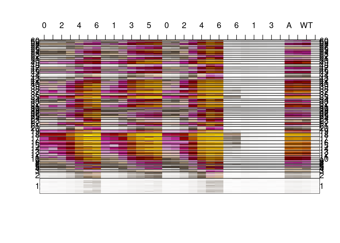
2.2.3 Figure 4B
options(repr.plot.width = 3, repr.plot.height = 20)
delta = m_s5[,c("d1_3a","d2_3a","d3_3a","d4_3a")]-
        m_s5[,c("d1_3b","d2_3b","d3_3b","d4_3b")]

dshades <- colorRampPalette(c("red","darkred","white","darkblue","blue"))(1000)
image(pmin(pmax(t(as.matrix(delta)),-0.3),0.3),col=dshades,zlim=c(-0.3,0.3))