6 Epigenomic instability

source(here::here("scripts/init.R"))

6.1 Compare features to each other

6.1 We change the direction (sign) of the clock and ML in order for it to be aligned with MG score, i.e. more progressed always equals higher score. This is implemented also in get_all_features() function.

feats_df_fixed <- fread(here("data/epigenomic_features.tsv")) %>% mutate(ML = -ML, clock = -clock) %>% as_tibble()

6.1.0.1 Figure 2E

options(repr.plot.width = 8, repr.plot.height = 4)
rho_pos <- cor(feats_df_fixed$MG[feats_df_fixed$ER == "ER+"], feats_df_fixed$ML[feats_df_fixed$ER == "ER+"], use="pairwise.complete.obs", method="spearman")
message(glue("rho ER+ = {rho_pos}"))

## rho ER+ = -0.166831861226654

p_MG_ML_scatter_ER_positive <- feats_df_fixed %>%     
    filter(ER == "ER+") %>% 
    ggplot(aes(x=MG, y=ML, color=ER)) + 
        geom_point(size=0.1) + 
        scale_color_manual(values = annot_colors$ER1) + 
        theme(aspect.ratio = 1) + 
        xlab("MG epigenomic instability") + 
        ylab("ML epigenomic instability") +         
        guides(color=FALSE) + 
        ggtitle("ER+")

## Warning: `guides(<scale> = FALSE)` is deprecated. Please use `guides(<scale> =
## "none")` instead.

rho_neg <- cor(feats_df_fixed$MG[feats_df_fixed$ER == "ER-"], feats_df_fixed$ML[feats_df_fixed$ER == "ER-"], use="pairwise.complete.obs", method="spearman")
message(glue("rho ER- = {rho_neg}"))

## rho ER- = -0.382303128930548

p_MG_ML_scatter_ER_negative <- feats_df_fixed %>%     
    filter(ER == "ER-") %>% 
    ggplot(aes(x=MG, y=ML, color=ER)) + 
        geom_point(size=0.1) + 
        scale_color_manual(values = annot_colors$ER1) + 
        theme(aspect.ratio = 1) + 
        xlab("MG epigenomic instability") + 
        ylab("ML epigenomic instability") +         
        guides(color=FALSE) + 
        ggtitle("ER-")

## Warning: `guides(<scale> = FALSE)` is deprecated. Please use `guides(<scale> =
## "none")` instead.

(p_MG_ML_scatter_ER_positive + theme_bw() + theme(aspect.ratio = 1)) + (p_MG_ML_scatter_ER_negative + theme_bw() + theme(aspect.ratio = 1))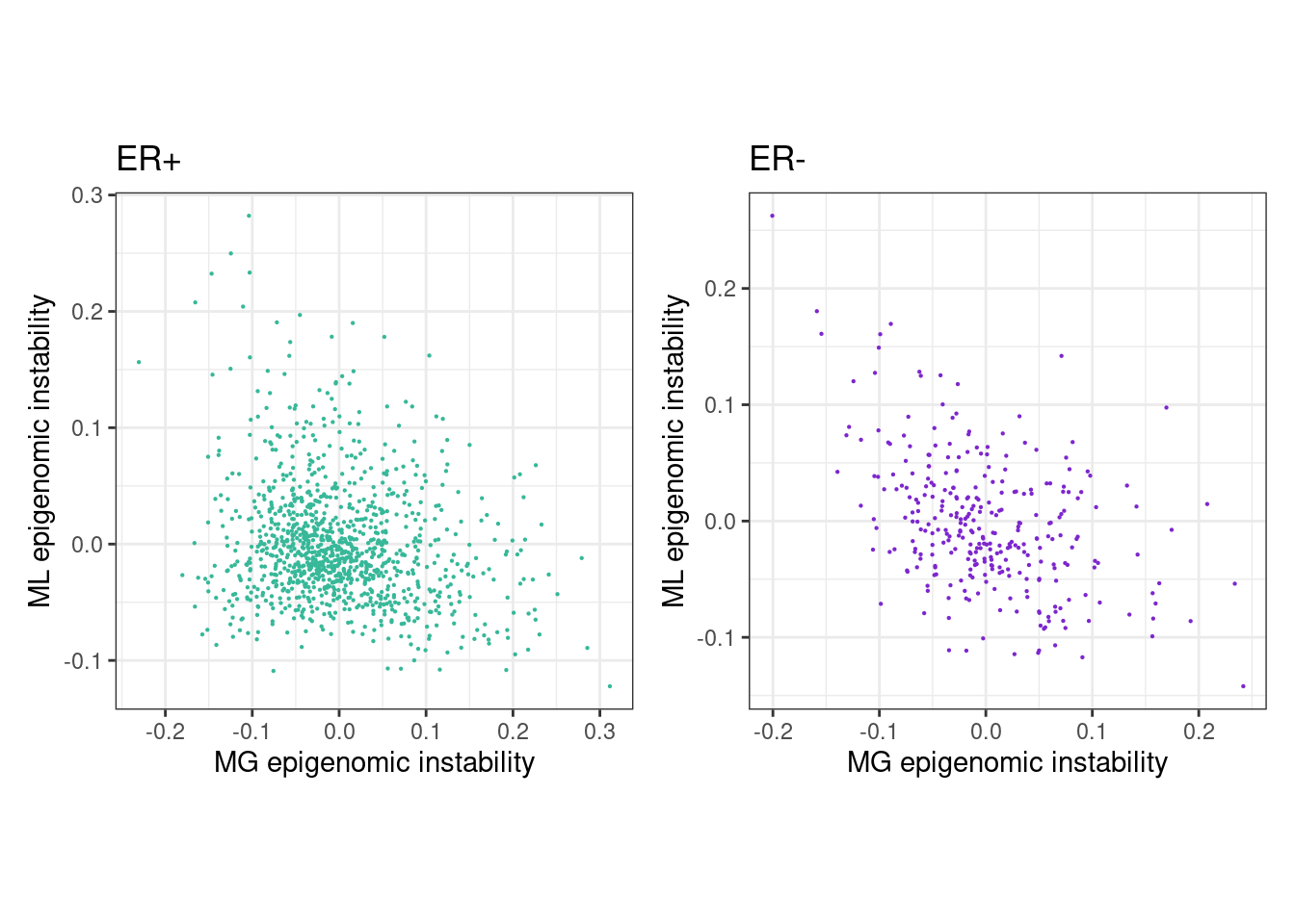

6.1.0.2 Extended Data Figure 6A

options(repr.plot.width = 8, repr.plot.height = 4)
rho_pos <- cor(feats_df_fixed$MG[feats_df_fixed$ER == "ER+"], feats_df_fixed$clock[feats_df_fixed$ER == "ER+"], use="pairwise.complete.obs", method="spearman")
message(glue("rho ER+ = {rho_pos}"))

## rho ER+ = -0.162654292782067

p_MG_clock_scatter_ER_positive <- feats_df_fixed %>%     
    filter(ER == "ER+") %>% 
    ggplot(aes(x=MG, y=clock, color=ER)) + 
        geom_point(size=0.1) + 
        scale_color_manual(values = annot_colors$ER1) + 
        theme(aspect.ratio = 1) + 
        xlab("MG epigenomic instability") + 
        ylab("Clock") + 
        guides(color=FALSE) + 
        ggtitle("ER+")

## Warning: `guides(<scale> = FALSE)` is deprecated. Please use `guides(<scale> =
## "none")` instead.

rho_neg <- cor(feats_df_fixed$MG[feats_df_fixed$ER == "ER-"], feats_df_fixed$clock[feats_df_fixed$ER == "ER-"], use="pairwise.complete.obs", method="spearman")
message(glue("rho ER- = {rho_neg}"))

## rho ER- = -0.28563668716636

p_MG_clock_scatter_ER_negative <- feats_df_fixed %>%     
    filter(ER == "ER-") %>% 
    ggplot(aes(x=MG, y=clock, color=ER)) + 
        geom_point(size=0.1) + 
        scale_color_manual(values = annot_colors$ER1) + 
        theme(aspect.ratio = 1) + 
        xlab("MG epigenomic instability") + 
        ylab("Clock") + 
        guides(color=FALSE) + 
        ggtitle("ER-")

## Warning: `guides(<scale> = FALSE)` is deprecated. Please use `guides(<scale> =
## "none")` instead.

(p_MG_clock_scatter_ER_positive + theme_bw() + theme(aspect.ratio = 1)) + (p_MG_clock_scatter_ER_negative + theme_bw() + theme(aspect.ratio = 1))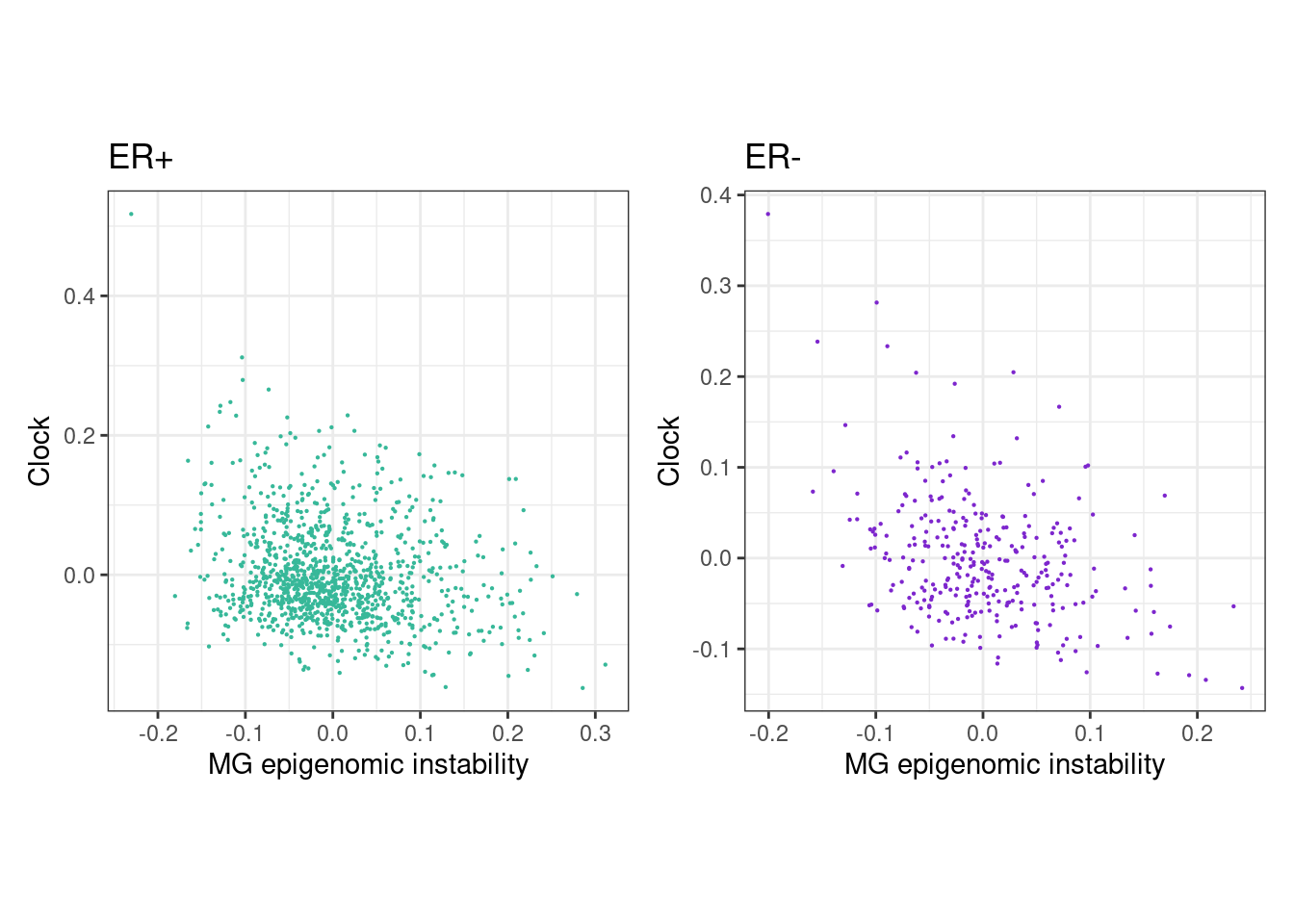

options(repr.plot.width = 8, repr.plot.height = 4)
rho_pos <- cor(feats_df_fixed$ML[feats_df_fixed$ER == "ER+"], feats_df_fixed$clock[feats_df_fixed$ER == "ER+"], use="pairwise.complete.obs", method="spearman")
message(glue("rho ER+ = {rho_pos}"))

## rho ER+ = 0.353548126048103

p_ML_clock_scatter_ER_positive <- feats_df_fixed %>%     
    filter(ER == "ER+") %>% 
    ggplot(aes(x=ML, y=clock, color=ER)) + 
        geom_point(size=0.1) + 
        scale_color_manual(values = annot_colors$ER1) + 
        theme(aspect.ratio = 1) + 
        xlab("ML epigenomic instability") + 
        ylab("Clock") + 
        guides(color=FALSE) + 
        ggtitle("ER+")

## Warning: `guides(<scale> = FALSE)` is deprecated. Please use `guides(<scale> =
## "none")` instead.

rho_neg <- cor(feats_df_fixed$ML[feats_df_fixed$ER == "ER-"], feats_df_fixed$clock[feats_df_fixed$ER == "ER-"], use="pairwise.complete.obs", method="spearman")
message(glue("rho ER- = {rho_neg}"))

## rho ER- = 0.64775559075671

p_ML_clock_scatter_ER_negative <- feats_df_fixed %>%     
    filter(ER == "ER-") %>% 
    ggplot(aes(x=ML, y=clock, color=ER)) + 
        geom_point(size=0.1) + 
        scale_color_manual(values = annot_colors$ER1) + 
        theme(aspect.ratio = 1) + 
        xlab("ML epigenomic instability") + 
        ylab("Clock") + 
        guides(color=FALSE) + 
        ggtitle("ER-")

## Warning: `guides(<scale> = FALSE)` is deprecated. Please use `guides(<scale> =
## "none")` instead.

(p_ML_clock_scatter_ER_positive + theme_bw() + theme(aspect.ratio = 1)) + (p_ML_clock_scatter_ER_negative + theme_bw() + theme(aspect.ratio = 1))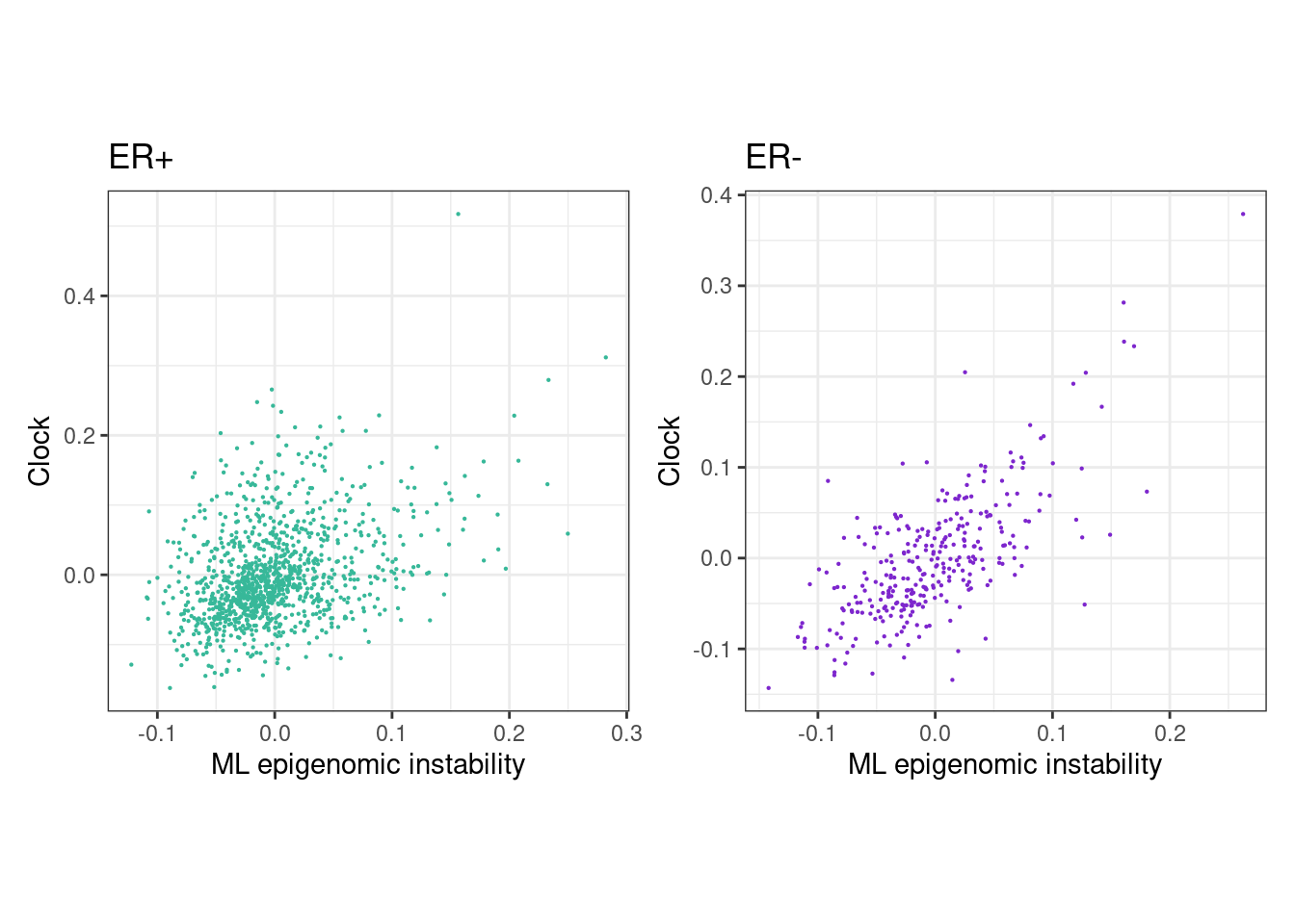

6.1.0.3 Extended Data Figure 6B

options(repr.plot.width = 8, repr.plot.height = 4)
rho_pos <- cor(feats_df_fixed$MG[feats_df_fixed$ER == "ER+"], feats_df_fixed$immune[feats_df_fixed$ER == "ER+"], use="pairwise.complete.obs", method="spearman")
message(glue("rho ER+ = {rho_pos}"))

## rho ER+ = 0.0256502058498626

p_MG_immune_scatter_ER_positive <- feats_df_fixed %>%     
    filter(ER == "ER+") %>% 
    ggplot(aes(x=MG, y=immune, color=ER)) + 
        geom_point(size=0.1) + 
        scale_color_manual(values = annot_colors$ER1) + 
        theme(aspect.ratio = 1) + 
        xlab("MG epigenomic instability") + 
        ylab("immune") + 
        guides(color=FALSE) + 
        ggtitle("ER+")

## Warning: `guides(<scale> = FALSE)` is deprecated. Please use `guides(<scale> =
## "none")` instead.

rho_neg <- cor(feats_df_fixed$MG[feats_df_fixed$ER == "ER-"], feats_df_fixed$immune[feats_df_fixed$ER == "ER-"], use="pairwise.complete.obs", method="spearman")
message(glue("rho ER- = {rho_neg}"))

## rho ER- = -0.0505710341049502

p_MG_immune_scatter_ER_negative <- feats_df_fixed %>%     
    filter(ER == "ER-") %>% 
    ggplot(aes(x=MG, y=immune, color=ER)) + 
        geom_point(size=0.1) + 
        scale_color_manual(values = annot_colors$ER1) + 
        theme(aspect.ratio = 1) + 
        xlab("MG epigenomic instability") + 
        ylab("immune") + 
        guides(color=FALSE) + 
        ggtitle("ER-")

## Warning: `guides(<scale> = FALSE)` is deprecated. Please use `guides(<scale> =
## "none")` instead.

(p_MG_immune_scatter_ER_positive + theme_bw() + theme(aspect.ratio = 1)) + (p_MG_immune_scatter_ER_negative + theme_bw() + theme(aspect.ratio = 1))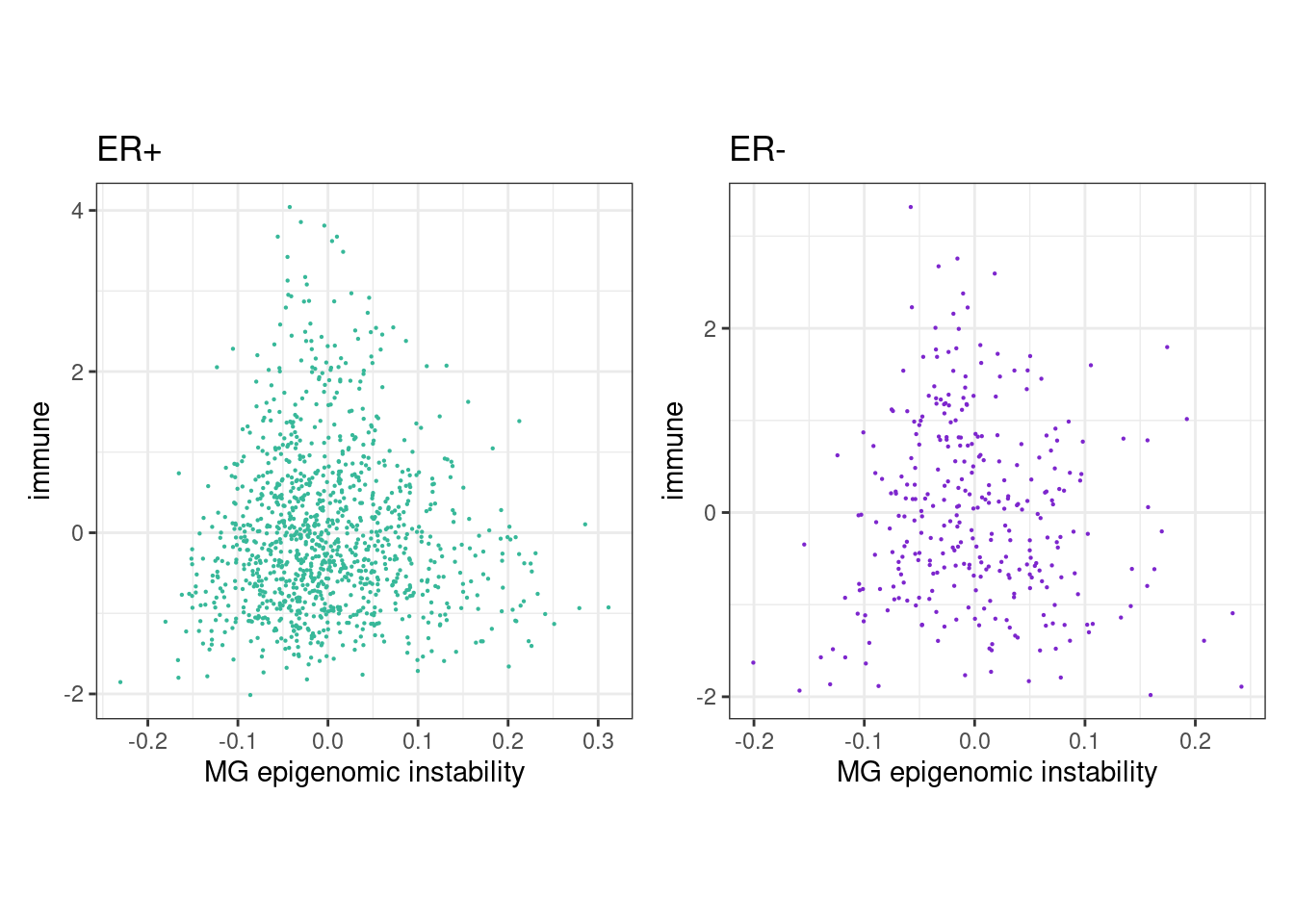

options(repr.plot.width = 8, repr.plot.height = 4)
rho_pos <- cor(feats_df_fixed$ML[feats_df_fixed$ER == "ER+"], feats_df_fixed$immune[feats_df_fixed$ER == "ER+"], use="pairwise.complete.obs", method="spearman")
message(glue("rho ER+ = {rho_pos}"))

## rho ER+ = 0.0182424884995677

p_ML_immune_scatter_ER_positive <- feats_df_fixed %>%     
    filter(ER == "ER+") %>% 
    ggplot(aes(x=ML, y=immune, color=ER)) + 
        geom_point(size=0.1) + 
        scale_color_manual(values = annot_colors$ER1) + 
        theme(aspect.ratio = 1) + 
        xlab("ML epigenomic instability") + 
        ylab("immune") + 
        guides(color=FALSE) + 
        ggtitle("ER+")

## Warning: `guides(<scale> = FALSE)` is deprecated. Please use `guides(<scale> =
## "none")` instead.

rho_neg <- cor(feats_df_fixed$ML[feats_df_fixed$ER == "ER-"], feats_df_fixed$immune[feats_df_fixed$ER == "ER-"], use="pairwise.complete.obs", method="spearman")
message(glue("rho ER- = {rho_neg}"))

## rho ER- = -0.0483692724136299

p_ML_immune_scatter_ER_negative <- feats_df_fixed %>%     
    filter(ER == "ER-") %>% 
    ggplot(aes(x=ML, y=immune, color=ER)) + 
        geom_point(size=0.1) + 
        scale_color_manual(values = annot_colors$ER1) + 
        theme(aspect.ratio = 1) + 
        xlab("ML epigenomic instability") + 
        ylab("immune") + 
        guides(color=FALSE) + 
        ggtitle("ER-")

## Warning: `guides(<scale> = FALSE)` is deprecated. Please use `guides(<scale> =
## "none")` instead.

(p_ML_immune_scatter_ER_positive + theme_bw() + theme(aspect.ratio = 1)) + (p_ML_immune_scatter_ER_negative + theme_bw() + theme(aspect.ratio = 1))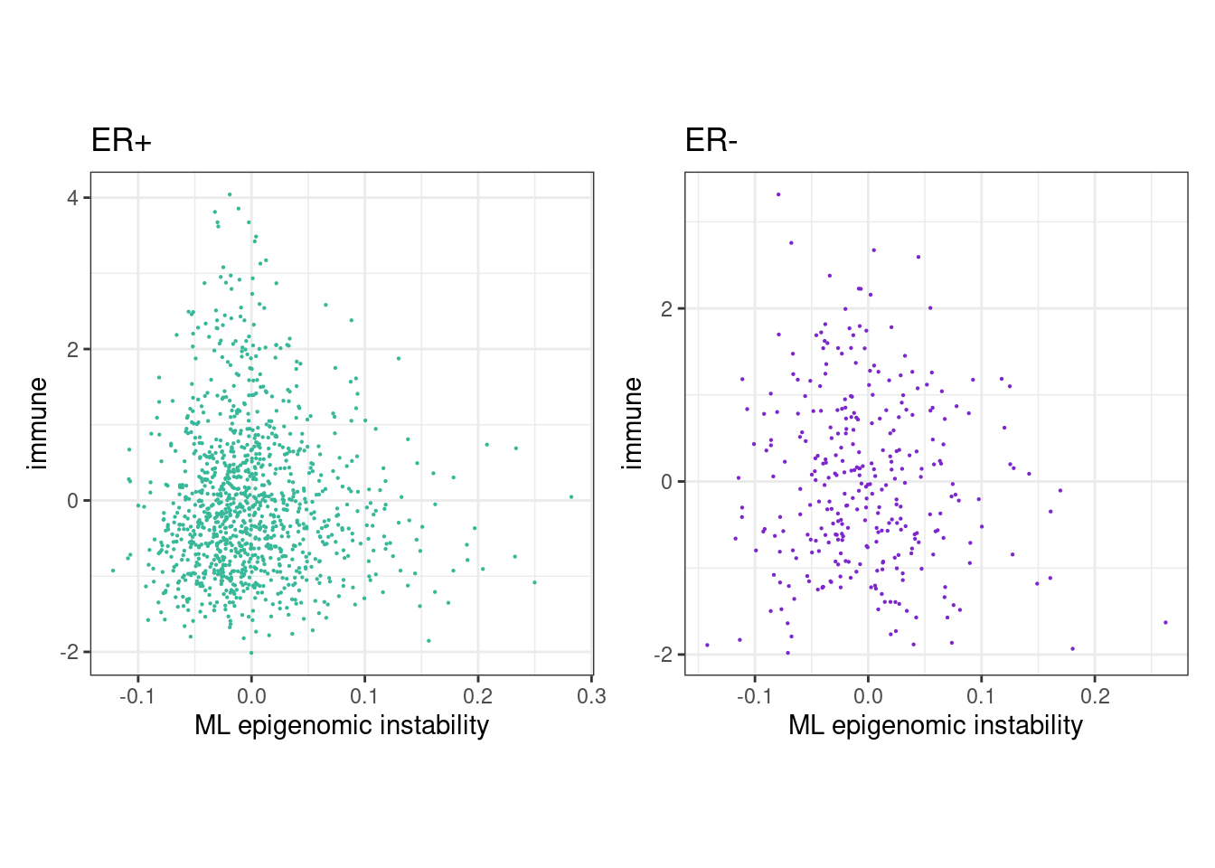

options(repr.plot.width = 8, repr.plot.height = 4)
rho_pos <- cor(feats_df_fixed$MG[feats_df_fixed$ER == "ER+"], feats_df_fixed$caf[feats_df_fixed$ER == "ER+"], use="pairwise.complete.obs", method="spearman")
message(glue("rho ER+ = {rho_pos}"))

## rho ER+ = 0.0201120969323973

p_MG_caf_scatter_ER_positive <- feats_df_fixed %>%     
    filter(ER == "ER+") %>% 
    ggplot(aes(x=MG, y=caf, color=ER)) + 
        geom_point(size=0.1) + 
        scale_color_manual(values = annot_colors$ER1) + 
        theme(aspect.ratio = 1) + 
        xlab("MG epigenomic instability") + 
        ylab("caf") + 
        guides(color=FALSE) + 
        ggtitle("ER+")

## Warning: `guides(<scale> = FALSE)` is deprecated. Please use `guides(<scale> =
## "none")` instead.

rho_neg <- cor(feats_df_fixed$MG[feats_df_fixed$ER == "ER-"], feats_df_fixed$caf[feats_df_fixed$ER == "ER-"], use="pairwise.complete.obs", method="spearman")
message(glue("rho ER- = {rho_neg}"))

## rho ER- = -0.00276791172007093

p_MG_caf_scatter_ER_negative <- feats_df_fixed %>%     
    filter(ER == "ER-") %>% 
    ggplot(aes(x=MG, y=caf, color=ER)) + 
        geom_point(size=0.1) + 
        scale_color_manual(values = annot_colors$ER1) + 
        theme(aspect.ratio = 1) + 
        xlab("MG epigenomic instability") + 
        ylab("caf") + 
        guides(color=FALSE) + 
        ggtitle("ER-")

## Warning: `guides(<scale> = FALSE)` is deprecated. Please use `guides(<scale> =
## "none")` instead.

(p_MG_caf_scatter_ER_positive + theme_bw() + theme(aspect.ratio = 1)) + (p_MG_caf_scatter_ER_negative + theme_bw() + theme(aspect.ratio = 1))

options(repr.plot.width = 8, repr.plot.height = 4)
rho_pos <- cor(feats_df_fixed$ML[feats_df_fixed$ER == "ER+"], feats_df_fixed$caf[feats_df_fixed$ER == "ER+"], use="pairwise.complete.obs", method="spearman")
message(glue("rho ER+ = {rho_pos}"))

## rho ER+ = 0.0336682666159654

p_ML_caf_scatter_ER_positive <- feats_df_fixed %>%     
    filter(ER == "ER+") %>% 
    ggplot(aes(x=ML, y=caf, color=ER)) + 
        geom_point(size=0.1) + 
        scale_color_manual(values = annot_colors$ER1) + 
        theme(aspect.ratio = 1) + 
        xlab("ML epigenomic instability") + 
        ylab("caf") + 
        guides(color=FALSE) + 
        ggtitle("ER+")

## Warning: `guides(<scale> = FALSE)` is deprecated. Please use `guides(<scale> =
## "none")` instead.

rho_neg <- cor(feats_df_fixed$ML[feats_df_fixed$ER == "ER-"], feats_df_fixed$caf[feats_df_fixed$ER == "ER-"], use="pairwise.complete.obs", method="spearman")
message(glue("rho ER- = {rho_neg}"))

## rho ER- = 0.0020186843607852

p_ML_caf_scatter_ER_negative <- feats_df_fixed %>%     
    filter(ER == "ER-") %>% 
    ggplot(aes(x=ML, y=caf, color=ER)) + 
        geom_point(size=0.1) + 
        scale_color_manual(values = annot_colors$ER1) + 
        theme(aspect.ratio = 1) + 
        xlab("ML epigenomic instability") + 
        ylab("caf") + 
        guides(color=FALSE) + 
        ggtitle("ER-")

## Warning: `guides(<scale> = FALSE)` is deprecated. Please use `guides(<scale> =
## "none")` instead.

(p_ML_caf_scatter_ER_positive + theme_bw() + theme(aspect.ratio = 1)) + (p_ML_caf_scatter_ER_negative + theme_bw() + theme(aspect.ratio = 1))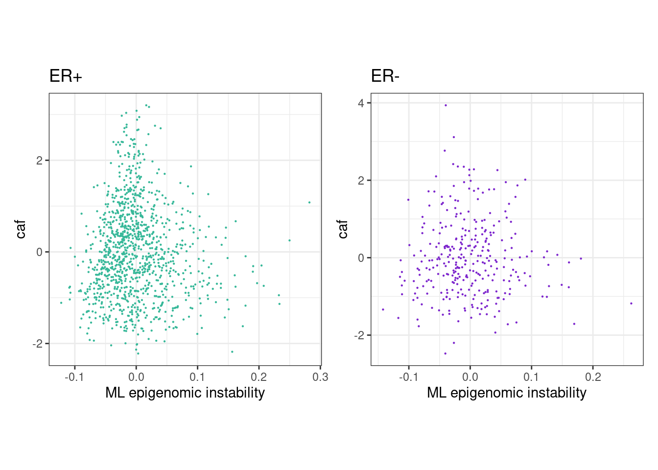

6.2 Annotate epignomic instability scores

feats <- get_all_features()
nbins <- 5
df <- feats %>% 
    mutate(
        clock = cut(clock, quantile(clock, 0:nbins/nbins, na.rm=TRUE), include.lowest=TRUE, labels=1:nbins), 
        immune = cut(immune, quantile(immune, 0:nbins/nbins, na.rm=TRUE), include.lowest=TRUE, labels=1:nbins), 
        caf = cut(caf, quantile(caf, 0:nbins/nbins, na.rm=TRUE), include.lowest=TRUE, labels=1:nbins), 
        immune.meth = cut(immune.meth, quantile(immune.meth, 0:nbins/nbins, na.rm=TRUE), include.lowest=TRUE, labels=1:nbins), 
        caf.meth = cut(caf.meth, quantile(caf.meth, 0:nbins/nbins, na.rm=TRUE), include.lowest=TRUE, labels=1:nbins), 
        MG = cut(MG, quantile(MG, 0:nbins/nbins, na.rm=TRUE), include.lowest=TRUE, labels=1:nbins), 
        ML = cut(ML, quantile(ML, 0:nbins/nbins, na.rm=TRUE), include.lowest=TRUE, labels=1:nbins)) %>% 
    left_join(samp_data %>% select(samp, stage, grade), by = "samp") %>% 
    mutate(stage = ifelse(stage %in% c(0, "DCIS", 1), "0-1", stage)) %>% 
    mutate(stage = ifelse(ER == "normal", "N", stage)) %>% 
    mutate(grade = ifelse(ER == "normal", "N", grade))

df_pval <- df %>% filter(ER %in% c("ER+", "ER-")) %>% gather("feat", "bin", -samp, -ER, -stage, -grade)  %>% group_by(ER, feat) %>% summarise(grade_pval = chisq.test(bin, grade)$p.value, stage_pval = chisq.test(bin, stage)$p.value) %>% mutate(signif_grade = case_when(grade_pval < 0.0001 ~ "****", grade_pval < 0.001 ~ "***", grade_pval < 0.01 ~ "**", grade_pval < 0.05 ~ "*"), signif_stage = case_when(stage_pval < 0.0001 ~ "****", stage_pval < 0.001 ~ "***",  stage_pval < 0.01 ~ "**", stage_pval < 0.05 ~ "*"))

## Warning in chisq.test(bin, grade): Chi-squared approximation may be incorrect

## Warning in chisq.test(bin, grade): Chi-squared approximation may be incorrect

## Warning in chisq.test(bin, grade): Chi-squared approximation may be incorrect

## Warning in chisq.test(bin, grade): Chi-squared approximation may be incorrect

## Warning in chisq.test(bin, grade): Chi-squared approximation may be incorrect

## Warning in chisq.test(bin, grade): Chi-squared approximation may be incorrect

## Warning in chisq.test(bin, grade): Chi-squared approximation may be incorrect

## Warning in chisq.test(bin, stage): Chi-squared approximation may be incorrect

## Warning in chisq.test(bin, stage): Chi-squared approximation may be incorrect

## Warning in chisq.test(bin, stage): Chi-squared approximation may be incorrect

## Warning in chisq.test(bin, stage): Chi-squared approximation may be incorrect

## Warning in chisq.test(bin, stage): Chi-squared approximation may be incorrect

## Warning in chisq.test(bin, stage): Chi-squared approximation may be incorrect

## Warning in chisq.test(bin, stage): Chi-squared approximation may be incorrect

## Warning in chisq.test(bin, stage): Chi-squared approximation may be incorrect

## Warning in chisq.test(bin, stage): Chi-squared approximation may be incorrect

## Warning in chisq.test(bin, stage): Chi-squared approximation may be incorrect

## Warning in chisq.test(bin, stage): Chi-squared approximation may be incorrect

## Warning in chisq.test(bin, stage): Chi-squared approximation may be incorrect

## Warning in chisq.test(bin, stage): Chi-squared approximation may be incorrect

as.data.frame(df_pval)

##     ER        feat   grade_pval  stage_pval signif_grade signif_stage
## 1  ER-         caf 2.264293e-04 0.001946125          ***           **
## 2  ER-    caf.meth 3.081915e-03 0.209690818           **         <NA>
## 3  ER-       clock 6.348596e-01 0.070940655         <NA>         <NA>
## 4  ER-      immune 3.712915e-01 0.580276177         <NA>         <NA>
## 5  ER- immune.meth 3.051790e-01 0.102242249         <NA>         <NA>
## 6  ER-          MG 5.763868e-01 0.042991948         <NA>            *
## 7  ER-          ML 6.479486e-01 0.873719290         <NA>         <NA>
## 8  ER+         caf 6.512545e-05 0.060334718         ****         <NA>
## 9  ER+    caf.meth 1.267372e-05 0.070515621         ****         <NA>
## 10 ER+       clock 1.471181e-01 0.572271776         <NA>         <NA>
## 11 ER+      immune 6.363196e-04 0.457202009          ***         <NA>
## 12 ER+ immune.meth 5.579626e-03 0.293001516           **         <NA>
## 13 ER+          MG 1.588818e-06 0.099708353         ****         <NA>
## 14 ER+          ML 5.428637e-10 0.230225194         ****         <NA>

df_pval %>% filter(grade_pval <= 0.05)

## # A tibble: 8 x 6
## # groups: ER
##    ER        feat    grade_pval  stage_pval signif_grade signif_stage
## 1 ER-         caf 0.00022642925 0.001946125          ***           **
## 2 ER-    caf.meth 0.00308191469 0.209690818           **         <NA>
## 3 ER+         caf 0.00006512545 0.060334718         ****         <NA>
## 4 ER+    caf.meth 0.00001267372 0.070515621         ****         <NA>
## 5 ER+      immune 0.00063631960 0.457202009          ***         <NA>
## 6 ER+ immune.meth 0.00557962596 0.293001516           **         <NA>
## # ... with 2 more rows

df_pval %>% filter(stage_pval <= 0.05)

## # A tibble: 2 x 6
## # groups: ER
##    ER feat   grade_pval  stage_pval signif_grade signif_stage
## 1 ER-  caf 0.0002264293 0.001946125          ***           **
## 2 ER-   MG 0.5763867809 0.042991948         <NA>            *

6.2.0.1 Extended Data Figure 6D

options(repr.plot.width = 6, repr.plot.height = 4)
p_stage_MG <- df %>% 
    filter(ER == "ER+") %>%
    mutate(stage = factor(stage, levels = c("N", "0-1", "2", "3", "4"))) %>% 
    filter(!is.na(stage)) %>% 
    count(stage, MG) %>% 
    group_by(MG) %>% 
    mutate(p = n / sum(n)) %>% 
    ggplot(aes(x=MG, y=p, fill=stage)) + 
        geom_col() + 
        scale_fill_manual(name = "Stage", values = c("N" = "gray", "0-1" = "black", "2" = "blue", "3" = "red", "4" = "orange")) + 
        scale_y_continuous(labels=scales::percent) + 
        ylab("% of samples")

p_stage_ML <- df %>% 
    filter(ER == "ER+") %>%
    mutate(stage = factor(stage, levels = c("N", "0-1", "2", "3", "4"))) %>% 
    filter(!is.na(stage)) %>% 
    count(stage, ML) %>% 
    group_by(ML) %>% 
    mutate(p = n / sum(n)) %>% 
    ggplot(aes(x=ML, y=p, fill=stage)) + 
        geom_col() + 
        scale_fill_manual(name = "Stage", values = c("N" = "gray", "0-1" = "black", "2" = "blue", "3" = "red", "4" = "orange")) + 
        scale_y_continuous(labels=scales::percent) + 
        ylab("% of samples")

p_stage_MG + theme_bw()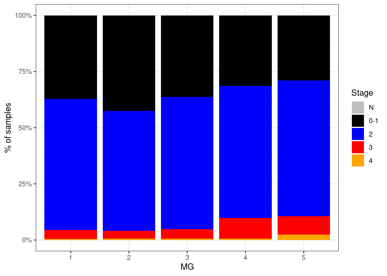

p_stage_ML + theme_bw()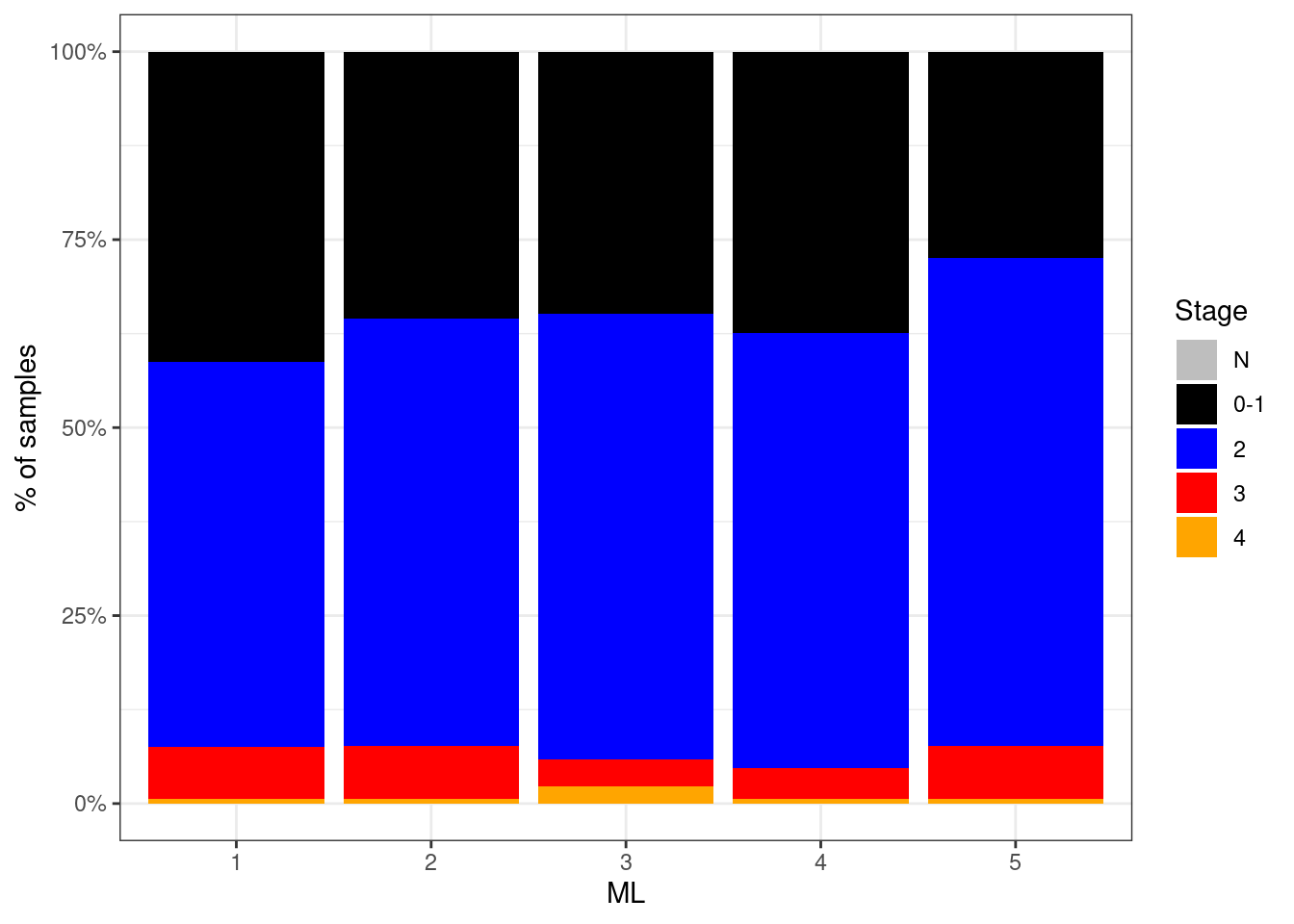

Same for ER-:

options(repr.plot.width = 6, repr.plot.height = 4)
p_grade_MG_neg <- df %>% 
    filter(ER == "ER-") %>%
    mutate(grade = factor(grade, levels = c("N", "1", "2", "3"))) %>% 
    filter(!is.na(grade)) %>% 
    count(grade, MG) %>% 
    group_by(MG) %>% 
    mutate(p = n / sum(n)) %>% 
    ggplot(aes(x=MG, y=p, fill=grade)) + 
        geom_col() + 
        scale_fill_manual(name = "Grade", values = c("N" = "gray", "1" = "darkblue", "2" = "red", "3" = "orange")) + 
        scale_y_continuous(labels=scales::percent) + 
        ylab("% of samples")

p_grade_ML_neg <- df %>% 
    filter(ER == "ER-") %>%
    mutate(grade = factor(grade, levels = c("N", "1", "2", "3"))) %>% 
    filter(!is.na(grade)) %>% 
    count(grade, ML) %>% 
    group_by(ML) %>% 
    mutate(p = n / sum(n)) %>% 
    ggplot(aes(x=ML, y=p, fill=grade)) + 
        geom_col() + 
        scale_fill_manual(name = "Grade", values = c("N" = "gray", "1" = "darkblue", "2" = "red", "3" = "orange")) + 
        scale_y_continuous(labels=scales::percent) + 
        ylab("% of samples")

p_grade_MG_neg + theme_bw()

p_grade_ML_neg + theme_bw()

options(repr.plot.width = 6, repr.plot.height = 4)
p_stage_MG_neg <- df %>% 
    filter(ER == "ER-") %>%
    mutate(stage = factor(stage, levels = c("N", "0-1", "2", "3", "4"))) %>% 
    filter(!is.na(stage)) %>% 
    count(stage, MG) %>% 
    group_by(MG) %>% 
    mutate(p = n / sum(n)) %>% 
    ggplot(aes(x=MG, y=p, fill=stage)) + 
        geom_col() + 
        scale_fill_manual(name = "Stage", values = c("N" = "gray", "0-1" = "black", "2" = "blue", "3" = "red", "4" = "orange")) + 
        scale_y_continuous(labels=scales::percent) + 
        ylab("% of samples")

p_stage_ML_neg <- df %>% 
    filter(ER == "ER-") %>%
    mutate(stage = factor(stage, levels = c("N", "0-1", "2", "3", "4"))) %>% 
    filter(!is.na(stage)) %>% 
    count(stage, ML) %>% 
    group_by(ML) %>% 
    mutate(p = n / sum(n)) %>% 
    ggplot(aes(x=ML, y=p, fill=stage)) + 
        geom_col() + 
        scale_fill_manual(name = "Stage", values = c("N" = "gray", "0-1" = "black", "2" = "blue", "3" = "red", "4" = "orange")) + 
        scale_y_continuous(labels=scales::percent) + 
        ylab("% of samples")

p_stage_MG_neg + theme_bw()

p_stage_ML_neg + theme_bw()

6.2.0.2 Figure 2D

options(repr.plot.width = 6, repr.plot.height = 4)
p_grade_MG <- df %>% 
    filter(ER == "ER+") %>%
    mutate(grade = factor(grade, levels = c("N", "1", "2", "3"))) %>% 
    filter(!is.na(grade)) %>% 
    count(grade, MG) %>% 
    group_by(MG) %>% 
    mutate(p = n / sum(n)) %>% 
    ggplot(aes(x=MG, y=p, fill=grade)) + 
        geom_col() + 
        scale_fill_manual(name = "Grade", values = c("N" = "gray", "1" = "darkblue", "2" = "red", "3" = "orange")) + 
        scale_y_continuous(labels=scales::percent) + 
        ylab("% of samples")

p_grade_ML <- df %>% 
    filter(ER == "ER+") %>%
    mutate(grade = factor(grade, levels = c("N", "1", "2", "3"))) %>% 
    filter(!is.na(grade)) %>% 
    count(grade, ML) %>% 
    group_by(ML) %>% 
    mutate(p = n / sum(n)) %>% 
    ggplot(aes(x=ML, y=p, fill=grade)) + 
        geom_col() + 
        scale_fill_manual(name = "Grade", values = c("N" = "gray", "1" = "darkblue", "2" = "red", "3" = "orange")) + 
        scale_y_continuous(labels=scales::percent) + 
        ylab("% of samples")

p_grade_MG + theme_bw()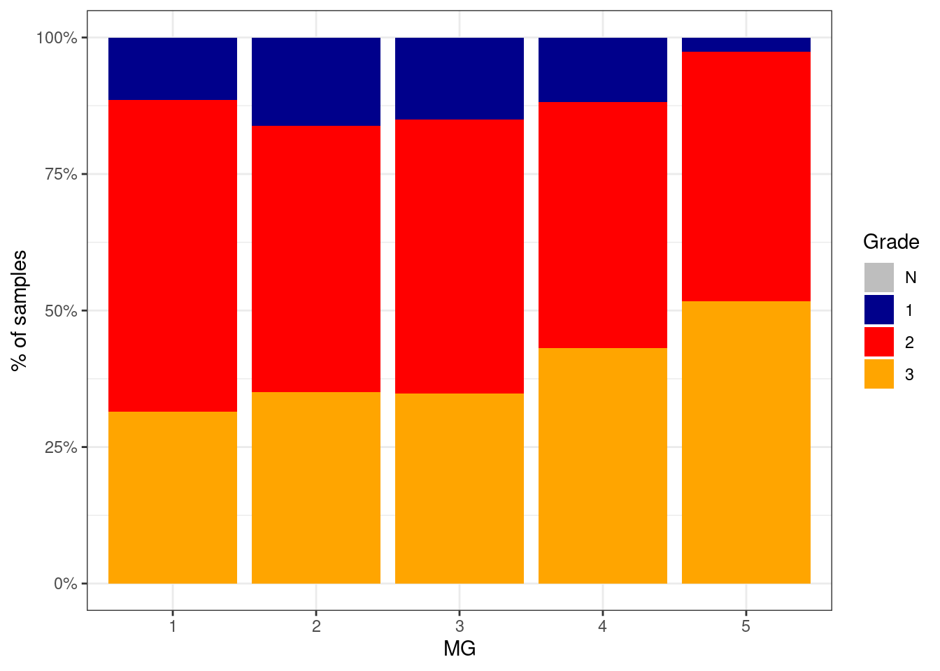

p_grade_ML + theme_bw()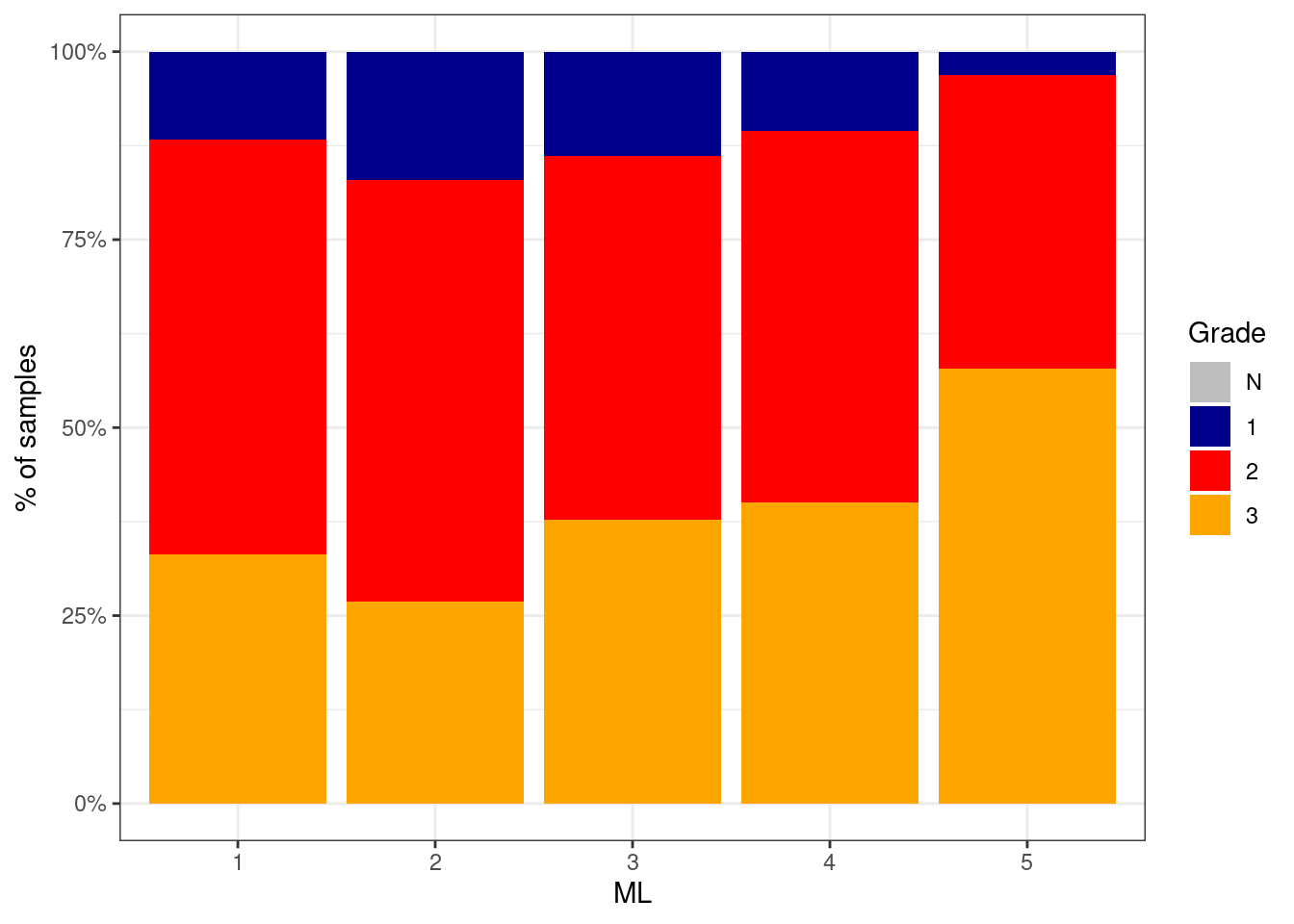

6.2.1 Integrative clusters

6.2.1.1 Extended Data Figure 7C

options(repr.plot.width = 8, repr.plot.height = 6)
df <- feats %>%
        left_join(samp_data %>% select(samp, iC10)) %>%
        filter(!is.na(iC10)) %>%
        mutate(iC10 = factor(iC10, levels = names(annot_colors$iC10))) %>%
        select(samp, ER, MG, ML, iC10) %>%
        gather("clust", "score", -ER, -iC10, -samp)

## Joining, by = "samp"

p_iC10 <- df %>%
        ggplot(aes(x = iC10, y = score, fill = iC10)) +
        geom_boxplot(lwd = 0.2, outlier.size = 0.2) +
        facet_grid(clust ~ .) +
        guides(fill = FALSE) +
        scale_fill_manual(values = annot_colors$iC10) +
        ylab("") +
        theme(aspect.ratio = 0.5) + 
        vertical_labs()

## Warning: `guides(<scale> = FALSE)` is deprecated. Please use `guides(<scale> =
## "none")` instead.

p_iC10 + theme_bw() + theme(aspect.ratio = 0.5) + vertical_labs() + ggpubr::stat_compare_means(method = "kruskal")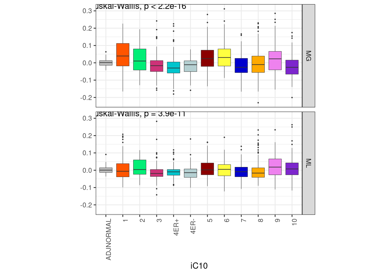

df %>% distinct(samp, iC10) %>% count(iC10)

## # A tibble: 12 x 2
##        iC10   n
## 1 ADJNORMAL  92
## 2         1  98
## 3         2  54
## 4         3 214
## 5      4ER+ 172
## 6      4ER-  50
## # ... with 6 more rows

6.3 Cross correlation (methylation-expression) of epigenomic instability loci

Create a matrix with methylation of loci that are part of MG or ML epigenmic instability and cross correlate it with gene expression in ER+:

all_norm_meth <- fread(here("data/all_norm_meth.tsv")) %>% as_tibble()
ER_positive_mat <- all_norm_meth %>% select(chrom:end, any_of(ER_positive_samples)) %>% intervs_to_mat()
loci_annot <- fread(here("data/loci_annot_epigenomic_features.tsv")) %>% as_tibble()
cor_thresh <- 0.3

coords <- loci_annot %>% 
    filter(abs(MG) >= cor_thresh | abs(ML) >= cor_thresh & abs(clock) < cor_thresh) %>% 
    select(chrom:end) %>% intervs_to_mat() %>% rownames()
meth_mat <- ER_positive_mat[coords, ]

expr_m <- fread(here("data/expression_matrix.csv")) %>% select(-any_of(c("chrom", "start", "end", "name3.chr")))
expr_mat <- expr_m %>%
    as.data.frame() %>%
    column_to_rownames("name")
f <- rowSums(!is.na(expr_mat)) > 0
expr_mat <- expr_mat[f, ]

em_cross <- em_cross_cor(meth_mat, expr_mat, meth_cor_thresh = 0.25, expr_cor_thresh = 0.25) %cache_rds% here("data/MG_ML_em_cross_cor.rds")

em_cross_clust <- cluster_em_cross_cor(em_cross, k_meth = 32, k_expr = 32) %cache_rds% here("data/MG_ML_em_cross_cor_clust.rds")

6.3.0.1 Figure 2F

options(repr.plot.width = 8, repr.plot.height = 13)
plot_em_cross_cor(em_cross_clust)

## plotting em cross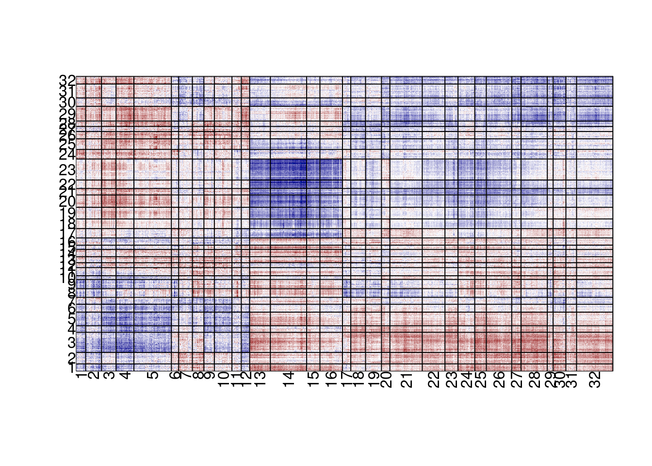

Annotating the methylation clusters we can see which are MG and which are ML

options(repr.plot.width = 10, repr.plot.height = 7)
cutree_order(em_cross_clust$hc_meth, k=32)  %>% 
    mat_to_intervs() %>% 
    set_names(c("chrom", "start", "end", "clust")) %>% 
    left_join(loci_annot %>% select(chrom, start, end,clock, MG, ML)) %>% 
    mutate(feat = case_when(
        clock >= cor_thresh ~ "clock", 
        MG >= cor_thresh ~ "MG", 
        ML >= cor_thresh ~ "ML", 
        TRUE ~ "other")) %>% 
    count(clust, feat)  %>% 
    as_tibble() %>% 
    group_by(clust) %>% 
    mutate(p = n / sum(n)) %>% 
    ggplot(aes(x=factor(clust), y=n, fill=feat)) + geom_col() + theme_bw()

## Joining, by = c("chrom", "start", "end")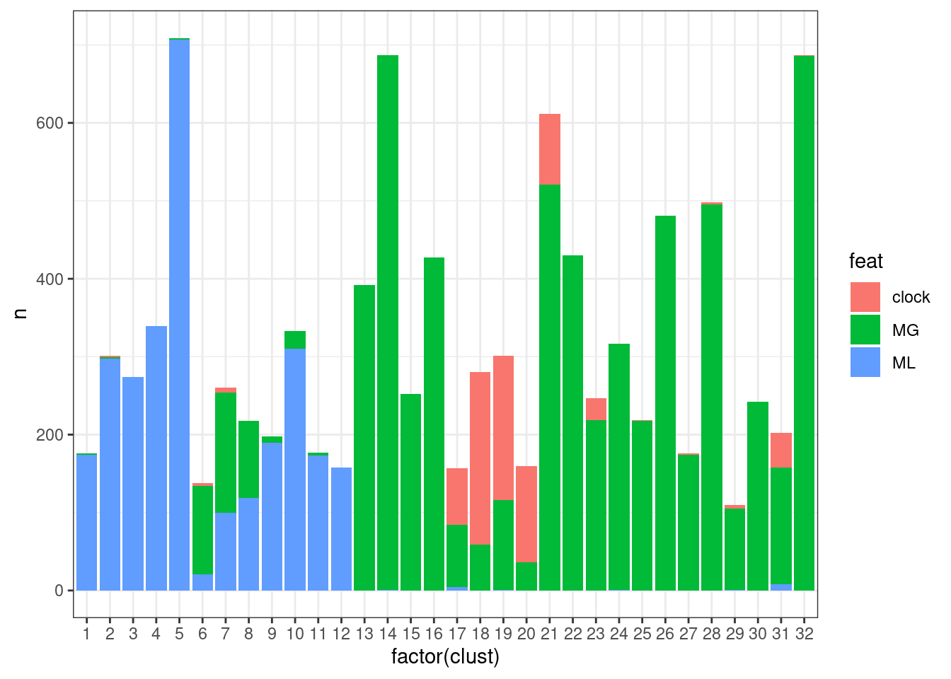

options(repr.plot.width = 8, repr.plot.height = 13)
plot_em_cross_cor(em_cross_clust, k_meth = 3, k_exp = 32)

## plotting em cross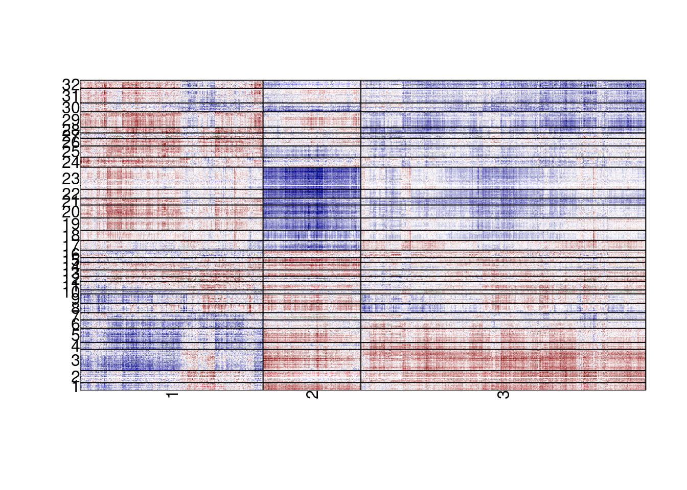

em_cross_clust$expr_clust %>% arrange(clust) %>% fwrite(here("data/MG_ML_em_cross_gene_clust_id.tsv"), sep="\t")

Plot for each expression cluster the name of the gene with highest correlation to any locus.

top_genes <- em_cross_clust$em_cross %>%
    gather_matrix("name", "locus", "cor") %>%
    left_join(em_cross_clust$expr_clust) %>%
    arrange(clust, cor) %>%
    group_by(clust) %>%
    slice(1) %>%
    ungroup() %>%
    left_join(em_cross_clust$expr_clust %>%
        count(clust) %>%
        mutate(p = cumsum(n / sum(n)), pos = p - (p - lag(p, default = 0)) / 2) %>%
        select(clust, pos)) %cache_df% here("data/MG_ML_em_cross_top_genes.tsv")

p_gene_names <- ggplot(top_genes, aes(x = 1, y = pos, label = name)) + geom_text() + theme_void(base_size = 3, base_family = "Arial")

Plot barplots of MG gene expression correlations

gene_annots <- get_gene_annots()

## Joining, by = "type"

feat_gene_cors <- get_expression_features_cors()

gene_annots_cors <- feat_gene_cors  %>% left_join(gene_annots, by = "name")  %>% filter(ER == "ER+", MG >= 0.15)  %>% distinct() 

6.3.0.2 Figure 2G

options(repr.plot.width = 8, repr.plot.height = 8)

p_cc <- gene_annots_cors %>%
        filter(type == "Cell Cycle") %>%
        ggplot(aes(x = reorder(name, MG), y = MG)) + geom_col(fill = "#008B45FF") + xlab("") + ylab("Correlation to MG") + vertical_labs() + ggtitle("Cell Cycle") + ylim(0, 0.5) + theme(axis.text.x = element_text(size = 4, family = "Arial")) + theme(plot.title = element_text(hjust = 0.5), panel.grid.major.x = element_blank())
p_emb <- gene_annots_cors %>%
        filter(type == "Embryonic TF") %>%
        ggplot(aes(x = reorder(name, MG), y = MG)) + geom_col(fill = "#3B4992FF") + xlab("") + ylab("Correlation to MG") + vertical_labs() + ggtitle("Embryonic TF") + ylim(0, 0.5) + theme(axis.text.x = element_text(size = 4, family = "Arial"), plot.title = element_text(hjust = 0.5), panel.grid.major.x = element_blank()) 
p_other <- gene_annots_cors %>%
        filter(type == "Other") %>%
        ggplot(aes(x = reorder(name, MG), y = MG)) + geom_col(fill = "black") + xlab("") + ylab("Correlation to MG") + vertical_labs() + ggtitle("Other") + ylim(0, 0.5) + theme(axis.text.x = element_text(size = 4, family = "Arial"), plot.title = element_text(hjust = 0.5), panel.grid.major.x = element_blank()) 

p_cc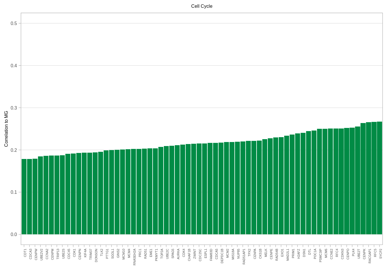

p_emb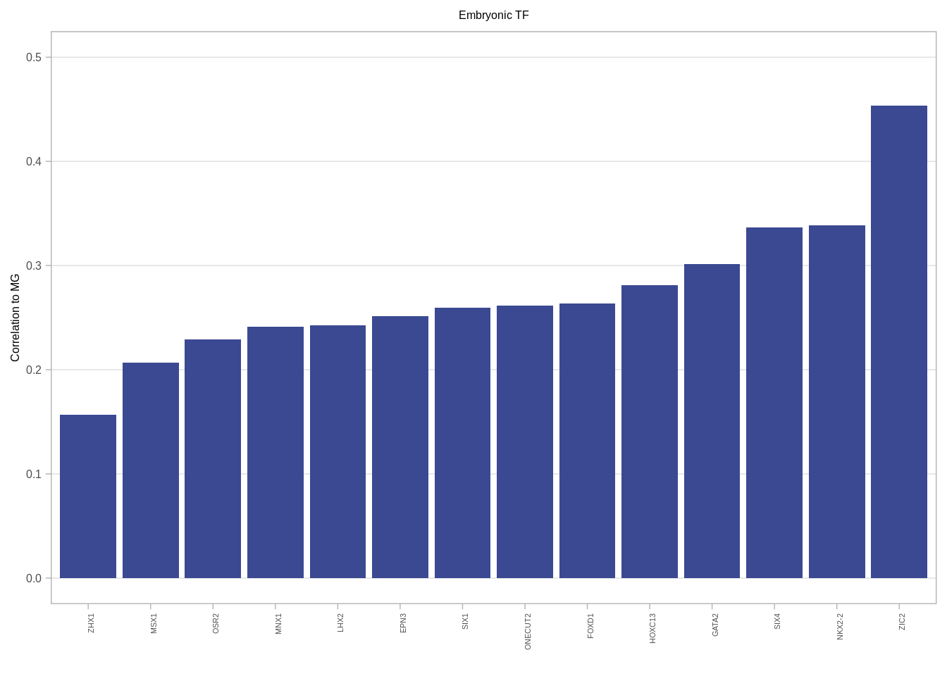

p_other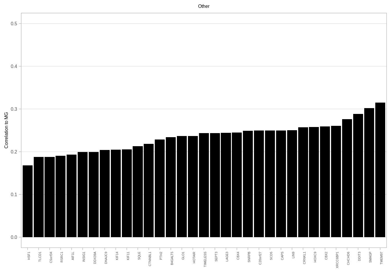

6.4 Epigenomic instability in different Time of replication (TOR) regimes

loci_annot <- fread(here("data/loci_annot_epigenomic_features.tsv")) %>% as_tibble()
loci_clust <- fread(here("data/ER_positive_loci_clust_df.tsv")) %>% as_tibble()
loci_clust <- loci_clust %>% left_join(loci_annot)

## Joining, by = c("chrom", "start", "end")

loci_clust_MG <- loci_clust %>% filter(clust == "MG")
loci_clust_ML <- loci_clust %>% filter(clust == "ML")

all_mat_raw <- get_all_meth() %>% intervs_to_mat()

tor_strata <- loci_clust_MG %>% mutate(tor_strata = cut(tor, breaks = main_config$genomic_regions$tor_low_mid_high, labels=c("late", "intermediate", "early"))) %>% pull(tor_strata) %>% forcats::fct_explicit_na()
intervs <- loci_clust_MG %>% intervs_to_mat() %>% rownames()

samp_meth_tor_MG <- tgs_matrix_tapply(t(all_mat_raw[intervs, ]), tor_strata, mean, na.rm=TRUE) %>% t() %>% as.data.frame() %>% rownames_to_column("samp") %>% add_ER() %>% as_tibble()

6.4.0.1 Extended Data Figure 7B

options(repr.plot.width = 4, repr.plot.height = 4)
p_early_late <- samp_meth_tor_MG %>% 
    filter(ER != "normal") %>% 
    ggplot(aes(x=early, y=late, color=ER)) + 
        geom_abline(linetype = "dashed") + 
        geom_point(size=0.5) + 
        xlim(0, 0.8) + 
        ylim(0, 0.8) + 
        xlab("MG loci: early replicating") + 
        ylab("MG loci: late replicating") + 
        scale_color_manual(values=annot_colors$ER1) +         
        theme(aspect.ratio = 1) 

samp_meth_tor_MG %>% filter(ER != "normal") %>% summarise(cor_early_late = cor(early, late, method = "spearman", use = "pairwise.complete.obs"), cor_early_mid = cor(early, intermediate, method = "spearman", use = "pairwise.complete.obs"))

## # A tibble: 1 x 2
##   cor_early_late cor_early_mid
## 1      0.8602804     0.9382058

p_early_late + theme_bw() + theme(aspect.ratio = 1)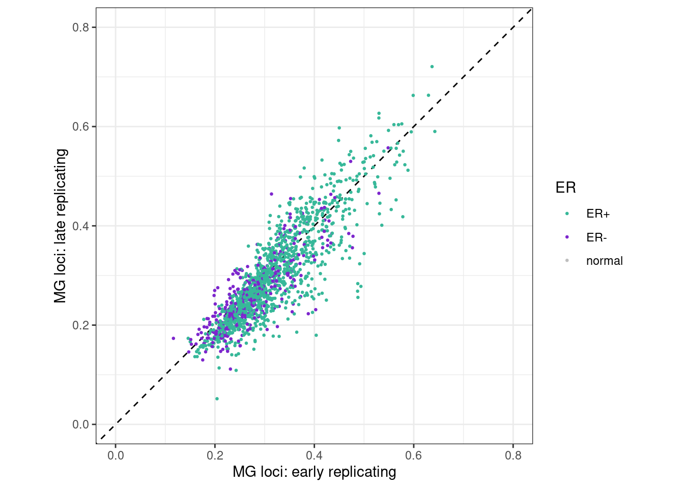 

tor_strata <- loci_clust_ML %>% mutate(tor_strata = cut(tor, breaks = main_config$genomic_regions$tor_low_mid_high, labels=c("late", "intermediate", "early"))) %>% pull(tor_strata) %>% forcats::fct_explicit_na()
intervs <- loci_clust_ML %>% intervs_to_mat() %>% rownames()

samp_meth_tor_ML <- tgs_matrix_tapply(t(all_mat_raw[intervs, ]), tor_strata, mean, na.rm=TRUE) %>% t() %>% as.data.frame() %>% rownames_to_column("samp") %>% add_ER() %>% as_tibble()

options(repr.plot.width = 4, repr.plot.height = 4)
p_early_late_ML <- samp_meth_tor_ML %>% 
    filter(ER != "normal") %>% 
    ggplot(aes(x=early, y=late, color=ER)) + 
        geom_abline(linetype = "dashed") + 
        geom_point(size=0.5) + 
        xlim(0, 0.8) + 
        ylim(0, 0.8) + 
        xlab("ML loci: early replicating") + 
        ylab("ML loci: late replicating") + 
        scale_color_manual(values=annot_colors$ER1) +         
        theme(aspect.ratio = 1) 

samp_meth_tor_ML %>% filter(ER != "normal") %>% summarise(cor_early_late = cor(early, late, method = "spearman", use = "pairwise.complete.obs"), cor_early_mid = cor(early, intermediate, method = "spearman", use = "pairwise.complete.obs"))

## # A tibble: 1 x 2
##   cor_early_late cor_early_mid
## 1      0.8201663     0.9276362

p_early_late_ML + theme_bw() + theme(aspect.ratio = 1) 

## Warning: Removed 32 rows containing missing values (geom_point).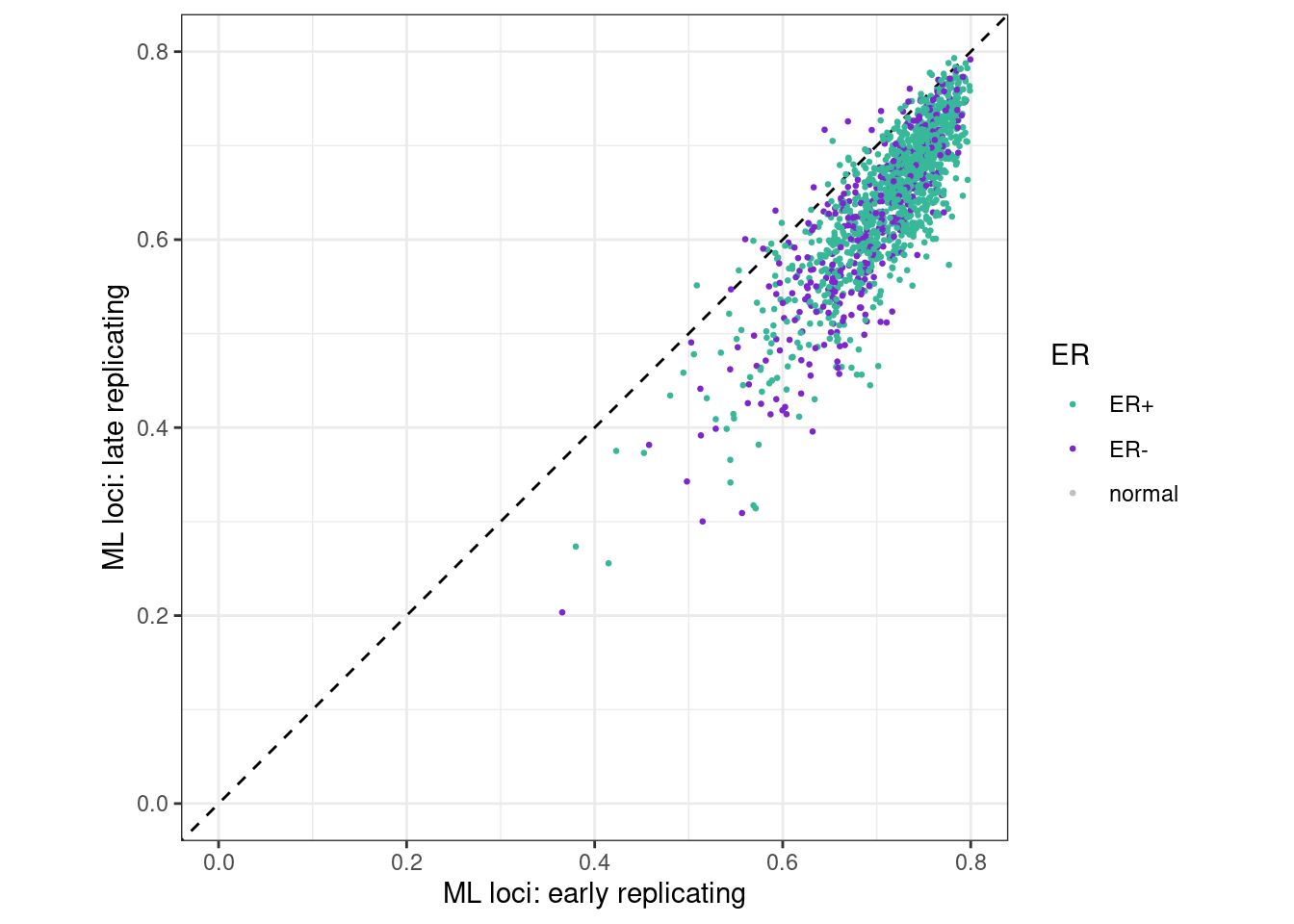

gc()

##              used    (Mb) gc trigger    (Mb)   max used    (Mb)
## Ncells    4690952   250.6    8042191   429.5    8042191   429.5
## Vcells 1417529451 10814.9 2192953529 16731.0 1803628477 13760.6