5 Loss clock

5.1 Introduction

We continue to characterize the highly correlated group of CpGs (see Epigenomic-scores notebook) we termed loss clock.

5.2 Initialize

source(here::here("scripts/init.R"))

5.3 Plot methylation distribution of the clock

df_sum <- fread(here("data/epigenomic_features_raw_meth.tsv")) %>% filter(!is.na(ER)) %>% as_tibble() 

5.3.0.1 Figure 1i

options(repr.plot.width = 4, repr.plot.height = 4)
p_avg_clock <- df_sum %>%         
    ggplot(aes(x=clock, color=ER)) + 
        geom_density() + 
        scale_color_manual(values = annot_colors$ER1) + 
        theme(aspect.ratio = 1) + 
        ylab("Density") + 
        xlab("Clock avg. methylation") + 
        coord_cartesian(xlim=c(0.4, 1))

p_avg_clock + theme_bw() + theme(aspect.ratio = 0.9)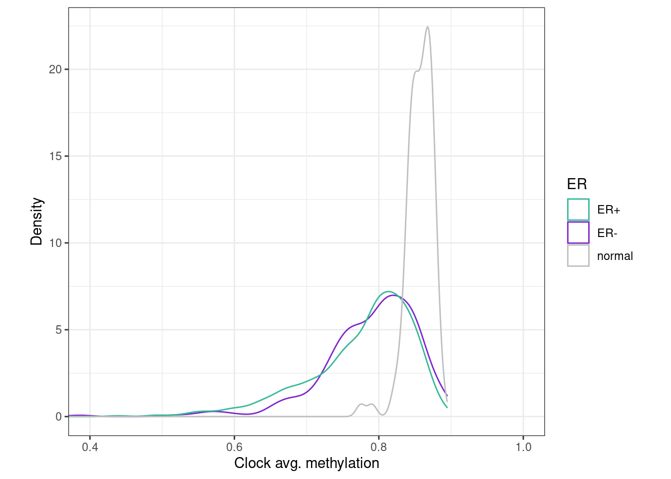    

ks.test(df_sum[df_sum$ER == "ER+", ]$clock, df_sum[df_sum$ER == "normal", ]$clock)

## 
##  Two-sample Kolmogorov-Smirnov test
## 
## data:  df_sum[df_sum$ER == "ER+", ]$clock and df_sum[df_sum$ER == "normal", ]$clock
## D = 0.73803, p-value < 2.2e-16
## alternative hypothesis: two-sided

ks.test(df_sum[df_sum$ER == "ER-", ]$clock, df_sum[df_sum$ER == "normal", ]$clock)

## 
##  Two-sample Kolmogorov-Smirnov test
## 
## data:  df_sum[df_sum$ER == "ER-", ]$clock and df_sum[df_sum$ER == "normal", ]$clock
## D = 0.68317, p-value < 2.2e-16
## alternative hypothesis: two-sided

5.4 Annotate "clock" score

5.4.1 Loci annotation

loci_annot <- fread(here("data/loci_annot_epigenomic_features.tsv")) %>% as_tibble()

cor_thresh <- 0.6

5.4.1.1 Figure 1k

options(repr.plot.width = 4, repr.plot.height = 4)
p_tss_d <- loci_annot %>% 
    mutate(type = ifelse(clock >= cor_thresh, "clock", "other")) %>% 
    ggplot(aes(x=abs(tss_d), color=type, linetype = type)) + 
    geom_density() + 
    xlab("Distance from TSS") + 
    ylab("Density") + 
    scale_color_manual(name = "", values=c(clock = "red", other = "gray")) + 
    scale_x_log10(label=scales::scientific) + 
    scale_linetype_manual(name = "", values=c(clock = "solid", other = "dashed")) + 
    theme(aspect.ratio = 0.8)

p_tss_d + theme_bw() + theme(aspect.ratio = 0.8)

## Warning: Transformation introduced infinite values in continuous x-axis

## Warning: Removed 21 rows containing non-finite values (stat_density).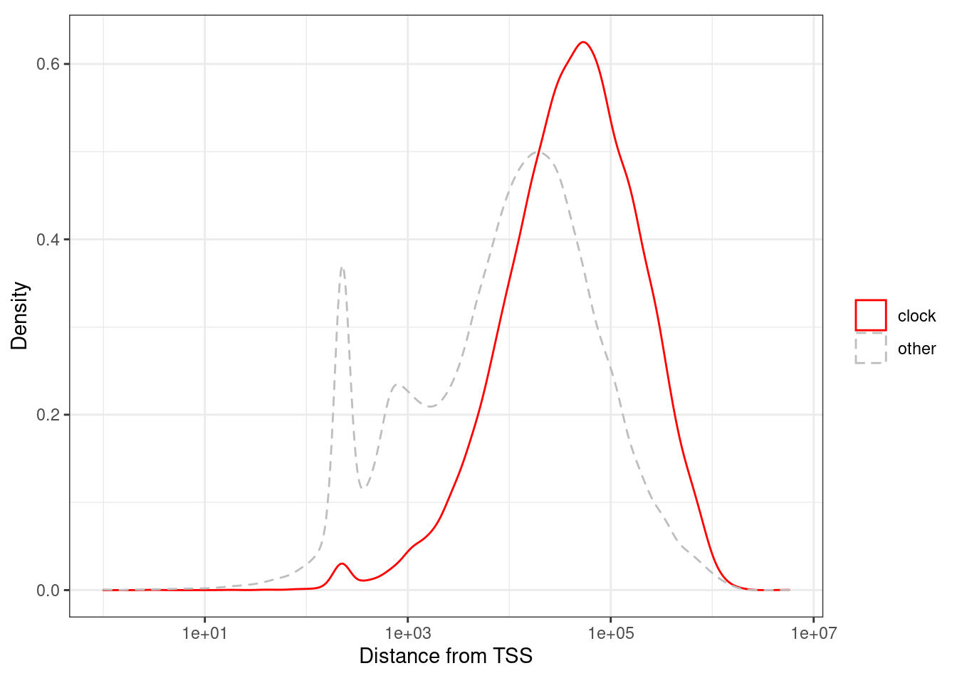

loci_annot %>% 
    mutate(type = ifelse(clock >= cor_thresh, "clock", "other")) %>% 
    summarise(pval = ks.test(abs(tss_d)[type == "clock"], abs(tss_d)[type == "other"])$p.value)

## Warning in ks.test(abs(tss_d)[type == "clock"], abs(tss_d)[type == "other"]): p-
## value will be approximate in the presence of ties

## # A tibble: 1 x 1
##   pval
## 1    0

5.4.1.2 Figure 1l

options(repr.plot.width = 4, repr.plot.height = 4)
p_tor <- loci_annot %>% 
    mutate(type = ifelse(clock >= cor_thresh, "clock", "other")) %>% 
    ggplot(aes(x=-tor, color=type, linetype = type)) + 
    geom_density() + 
    xlab("Time of replication") + 
    ylab("Density") + 
    scale_color_manual(name = "", values=c(clock = "red", other = "gray")) + 
    scale_x_continuous(breaks = c(-80, 0), labels = c("Early", "Late")) + 
    scale_linetype_manual(name = "", values=c(clock = "solid", other = "dashed")) + 
    theme(aspect.ratio = 0.8)

p_tor  + theme_bw() + theme(aspect.ratio = 0.8)

## Warning: Removed 28 rows containing non-finite values (stat_density).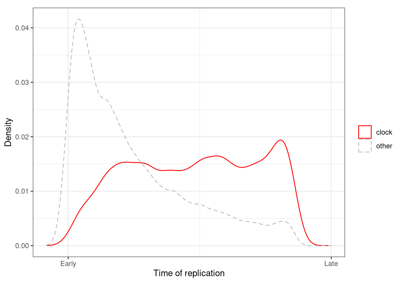

loci_annot %>% 
    mutate(type = ifelse(clock >= cor_thresh, "clock", "other")) %>% 
    summarise(pval = ks.test(-tor[type == "clock"], -tor[type == "other"])$p.value)

## Warning in ks.test(-tor[type == "clock"], -tor[type == "other"]): p-value will
## be approximate in the presence of ties

## # A tibble: 1 x 1
##   pval
## 1    0

5.4.1.3 Extended Data Figure 4d

options(repr.plot.width = 4, repr.plot.height = 4)
p_cg_cont_d <- loci_annot %>% 
    mutate(type = ifelse(clock >= cor_thresh, "clock", "other")) %>% 
    ggplot(aes(x=cg_cont, color=type, linetype = type)) + 
    geom_density() + 
    xlab("CpG content (500bp)") + 
    ylab("Density") + 
    scale_color_manual(name = "", values=c(clock = "red", other = "gray")) + 
    scale_linetype_manual(name = "", values=c(clock = "solid", other = "dashed")) + 
    theme(aspect.ratio = 0.8)

p_cg_cont_d + theme_bw() + theme(aspect.ratio = 0.8)

## Warning: Removed 8 rows containing non-finite values (stat_density).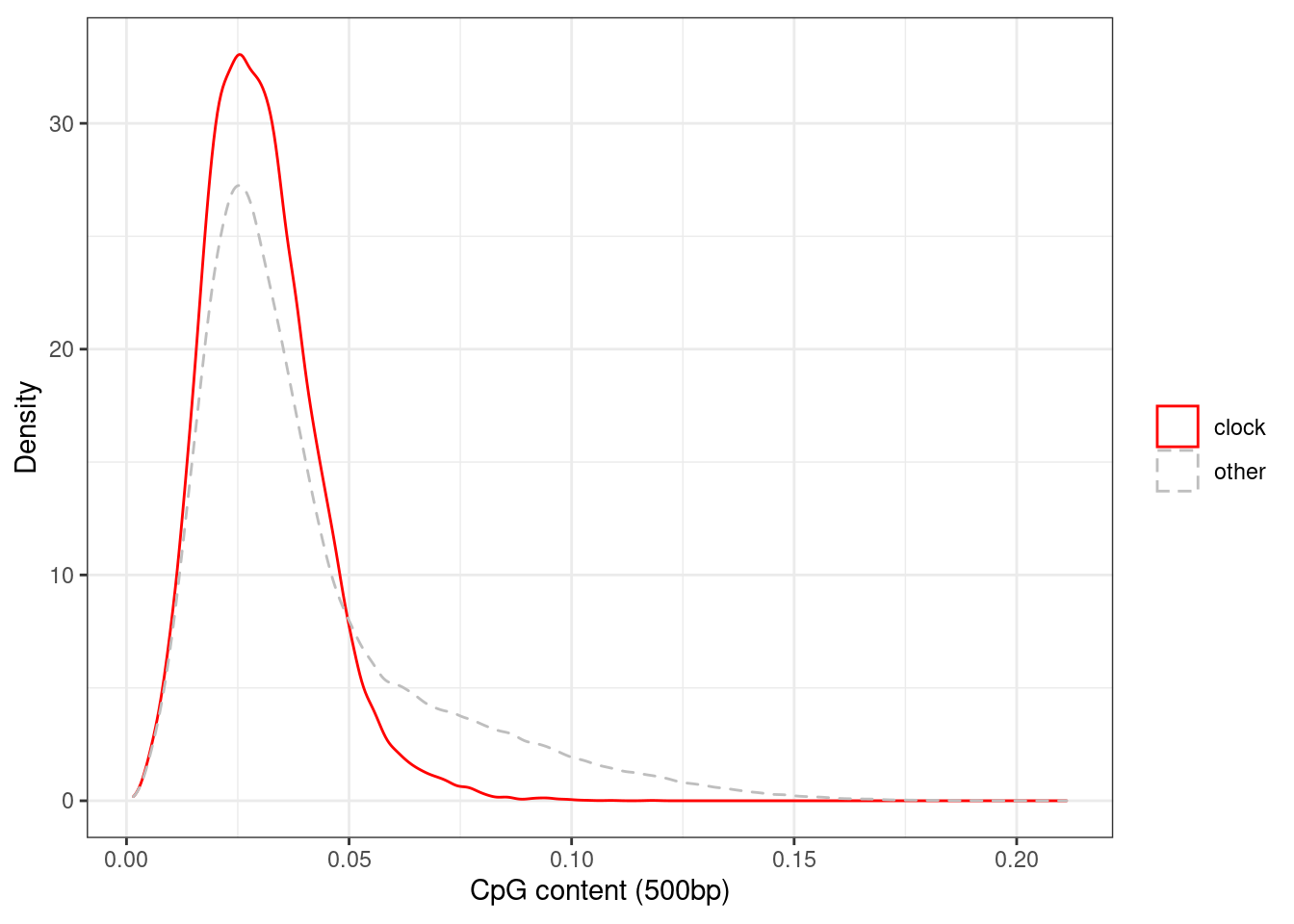

loci_annot %>% 
    mutate(type = ifelse(clock >= cor_thresh, "clock", "other")) %>% 
    summarise(pval = ks.test(cg_cont[type == "clock"], cg_cont[type == "other"])$p.value)

## Warning in ks.test(cg_cont[type == "clock"], cg_cont[type == "other"]): p-value
## will be approximate in the presence of ties

## # A tibble: 1 x 1
##   pval
## 1    0

5.4.1.4 Extended Data Figure 4c

options(repr.plot.width = 4, repr.plot.height = 4)

k4me1_names <- grep("k4me1", colnames(loci_annot))

clock_loci_annot <- loci_annot %>%
        mutate(type = ifelse(clock >= cor_thresh, "clock", "other")) %>%
        mutate(
            enh = matrixStats::rowAnys((loci_annot[, k4me1_names] > 0.97), na.rm = TRUE),
            polycomb = k27me3 > 0.97
        ) %>%
        mutate(context = case_when(polycomb ~ "K27me3 peaks", enh ~ "K4me1 peaks", TRUE ~ "Background"))

p_enh_polycomb <- clock_loci_annot %>%
        count(type, context) %>%
        group_by(type) %>%
        mutate(frac = n / sum(n)) %>%
        ggplot(aes(x = context, y = frac, fill = type)) +
        geom_col(position = "dodge") +
        scale_fill_manual("", values = c(other = "gray", clock = "red")) +
        scale_y_continuous(label = function(x) scales::percent(x, accuracy = 1)) +
        ylab("Percent of sites") +
        xlab("") +
        guides(fill = FALSE) +
        vertical_labs() +
        theme(aspect.ratio = 0.8)

## Warning: `guides(<scale> = FALSE)` is deprecated. Please use `guides(<scale> =
## "none")` instead.

p_enh_polycomb + theme_bw() + theme(aspect.ratio = 0.8)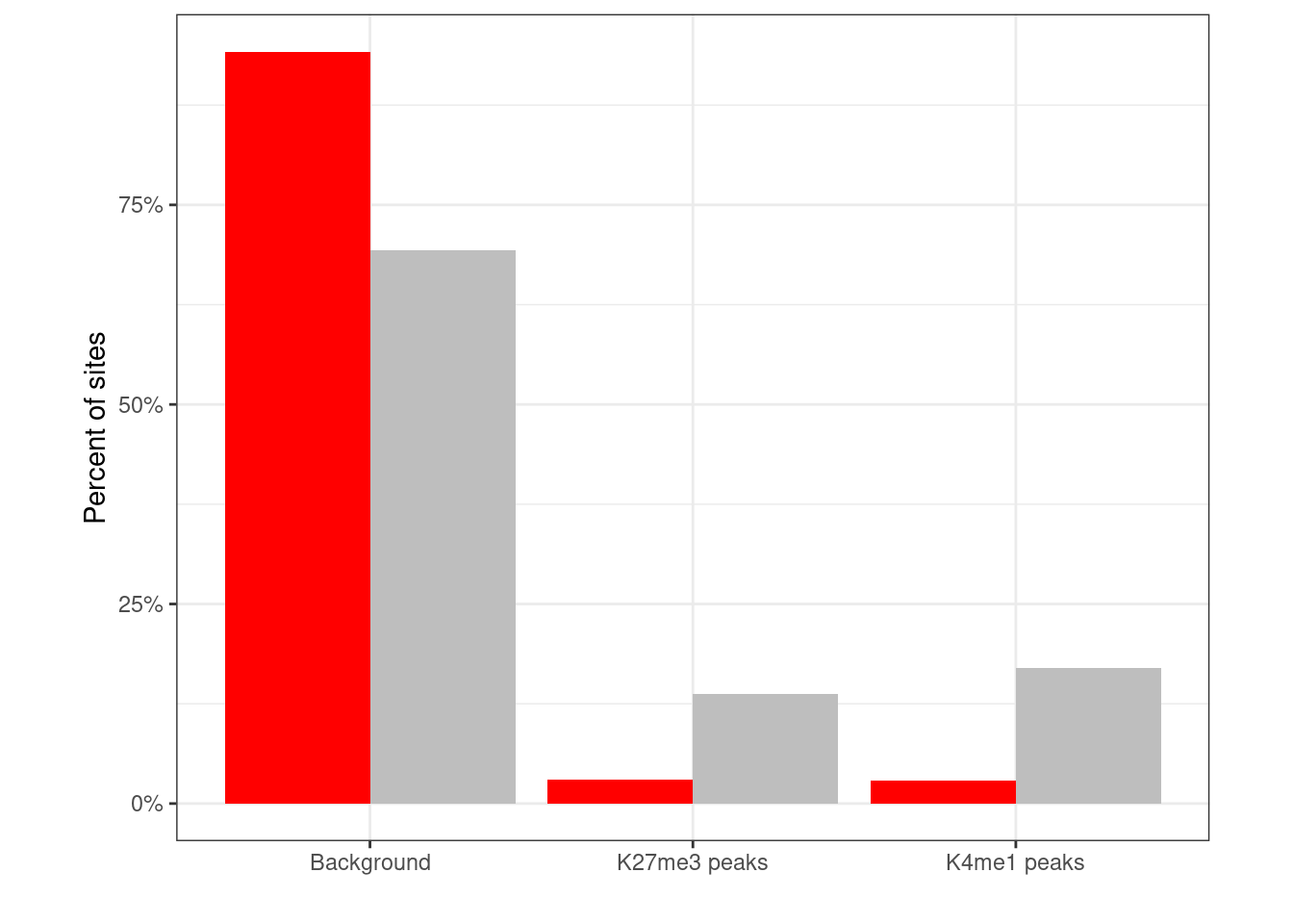

chisq.test(clock_loci_annot$type, clock_loci_annot$context)

## 
##  Pearson's Chi-squared test
## 
## data:  clock_loci_annot$type and clock_loci_annot$context
## X-squared = 4794, df = 2, p-value < 2.2e-16

5.4.2 Clinical annotation

feats <- fread(here("data/epigenomic_features.tsv")) %>% 
        mutate(ML = -ML, clock = -clock, immune.meth = -immune.meth, caf.meth = -caf.meth) %>% as_tibble()
nbins <- 5
df <- feats %>% 
    mutate(
        clock = cut(clock, quantile(clock, 0:nbins/nbins, na.rm=TRUE), include.lowest=TRUE, labels=1:nbins)) %>% 
    left_join(samp_data %>% select(samp, stage, grade), by = "samp") %>% 
    mutate(stage = ifelse(stage %in% c(0, "DCIS", 1), "0-1", stage)) %>% 
    mutate(stage = ifelse(ER == "normal", "N", stage)) %>% 
    mutate(grade = ifelse(ER == "normal", "N", grade))

df_pval <- df %>% filter(ER %in% c("ER+", "ER-")) %>% gather("feat", "bin", -samp, -ER, -stage, -grade) %>% filter(feat == "clock") %>% group_by(ER, feat) %>% summarise(grade_pval = chisq.test(bin, grade)$p.value, stage_pval = chisq.test(bin, stage)$p.value) 

## Warning: attributes are not identical across measure variables;
## they will be dropped

## Warning in chisq.test(bin, grade): Chi-squared approximation may be incorrect

## Warning in chisq.test(bin, stage): Chi-squared approximation may be incorrect

## Warning in chisq.test(bin, stage): Chi-squared approximation may be incorrect

as.data.frame(df_pval)

##    ER  feat grade_pval stage_pval
## 1 ER- clock  0.6348596 0.07094066
## 2 ER+ clock  0.1471181 0.57227178

df_pval %>% filter(grade_pval <= 0.05)

## # A tibble: 0 x 4
## # groups: ER
## [1] ER         feat       grade_pval stage_pval
## <0 rows> (or 0-length row.names)

df_pval %>% filter(stage_pval <= 0.05)

## # A tibble: 0 x 4
## # groups: ER
## [1] ER         feat       grade_pval stage_pval
## <0 rows> (or 0-length row.names)

options(repr.plot.width = 6, repr.plot.height = 4)
p_stage_clock <- df %>% 
    filter(ER == "ER+") %>%
    mutate(stage = factor(stage, levels = c("N", "0-1", "2", "3", "4"))) %>% 
    filter(!is.na(stage)) %>% 
    count(stage, clock) %>% 
    group_by(clock) %>% 
    mutate(p = n / sum(n)) %>% 
    ggplot(aes(x=clock, y=p, fill=stage)) + 
        geom_col() + 
        scale_fill_manual(name = "Stage", values = c("N" = "gray", "0-1" = "black", "2" = "blue", "3" = "red", "4" = "orange")) + 
        scale_y_continuous(labels=scales::percent) + 
        ylab("% of samples")

p_stage_clock + theme_bw()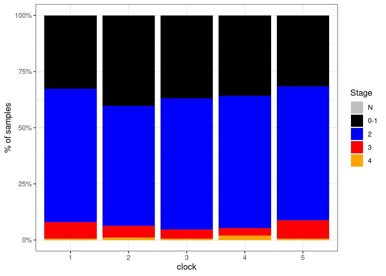

5.4.2.1 Figure 1j

options(repr.plot.width = 6, repr.plot.height = 4)
p_grade_clock_positive <- df %>% 
    filter(ER == "ER+") %>%
    mutate(grade = factor(grade, levels = c("N", "1", "2", "3"))) %>% 
    filter(!is.na(grade)) %>% 
    count(grade, clock) %>% 
    group_by(clock) %>% 
    mutate(p = n / sum(n)) %>% 
    ggplot(aes(x=clock, y=p, fill=grade)) + 
        geom_col() + 
        scale_fill_manual(name = "Grade", values = c("N" = "gray", "1" = "darkblue", "2" = "red", "3" = "orange")) + 
        scale_y_continuous(labels=scales::percent) + 
        ylab("% of samples")

p_grade_clock_negative <- df %>% 
    filter(ER == "ER-") %>%
    mutate(grade = factor(grade, levels = c("N", "1", "2", "3"))) %>% 
    filter(!is.na(grade)) %>% 
    count(grade, clock) %>% 
    group_by(clock) %>% 
    mutate(p = n / sum(n)) %>% 
    ggplot(aes(x=clock, y=p, fill=grade)) + 
        geom_col() + 
        scale_fill_manual(name = "Grade", values = c("N" = "gray", "1" = "darkblue", "2" = "red", "3" = "orange")) + 
        scale_y_continuous(labels=scales::percent) + 
        ylab("% of samples")

p_grade_clock_positive + theme_bw()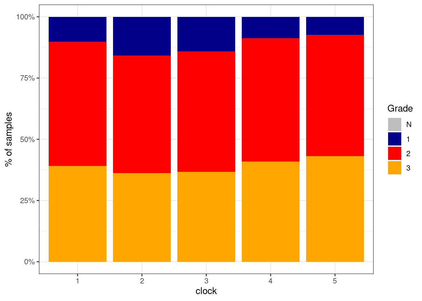

p_grade_clock_negative + theme_bw()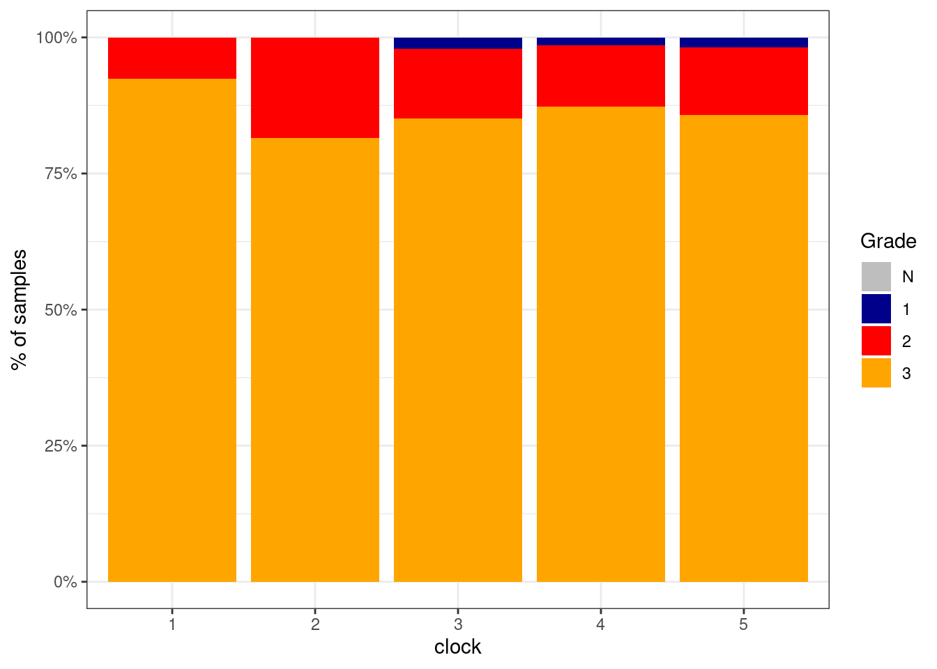

5.5 Plot chromosomal traces of clock score

We separate the samples to tumors with high and low clock score (top and bottom 30%). We then look at average methylation in bins of 10K along the chromosome.
We smooth the methylation traces with rolling average of 50 bins.

5.5.0.1 Figure 1m

options(repr.plot.width = 14, repr.plot.height = 5)
p_trace <- plot_tor_clock_chrom_track("chr1", "ER+", iterator=1e4)

## Warning: `guides(<scale> = FALSE)` is deprecated. Please use `guides(<scale> =
## "none")` instead.

## Warning: `guides(<scale> = FALSE)` is deprecated. Please use `guides(<scale> =
## "none")` instead.

## Warning: Removed 147 row(s) containing missing values (geom_path).

p_trace$p + coord_cartesian(ylim = c(0.25, 0.77))

## Coordinate system already present. Adding new coordinate system, which will replace the existing one.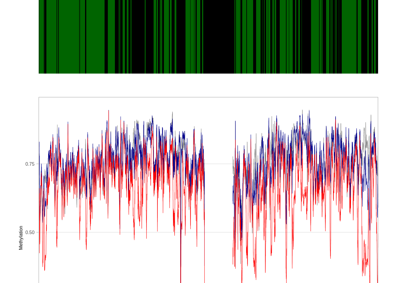

5.5.0.2 Extended Data Figure 4f

options(repr.plot.width = 14, repr.plot.height = 5)
p_trace_chr10 <- plot_tor_clock_chrom_track("chr10", "ER+", iterator=1e4)

## Warning: `guides(<scale> = FALSE)` is deprecated. Please use `guides(<scale> =
## "none")` instead.

## Warning: `guides(<scale> = FALSE)` is deprecated. Please use `guides(<scale> =
## "none")` instead.

## Warning: Removed 147 row(s) containing missing values (geom_path).

p_trace_chr10$p + coord_cartesian(ylim = c(0.1, 0.77))

## Coordinate system already present. Adding new coordinate system, which will replace the existing one.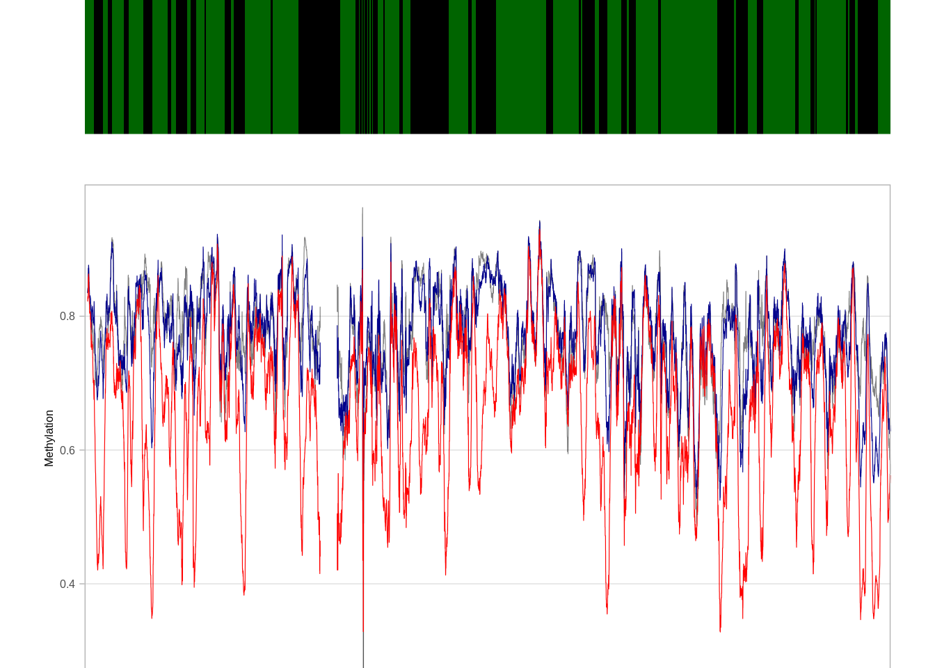

5.6 Correlation of gene expression to clock

We calculate the correlation of all the genes to the clock score.

feat_gene_cors <- get_expression_features_cors()

5.6.0.1 Extended Data Figure 5a

options(repr.plot.width = 4, repr.plot.height = 7)

top_genes <- feat_gene_cors %>%
    filter(ER == "ER+") %>%
    arrange(-clock) %>%
    slice(1:25)
p_top_genes <- top_genes %>%
    ggplot(aes(x = reorder(name, clock), y = clock, fill = ER)) +
    geom_col() +
    scale_fill_manual("", values = annot_colors$ER1) +
    guides(fill = "none") +
    ylim(0, 0.5) +
    xlab("") +
    ylab("ER+") + 
    coord_flip() + 
    ggtitle("Correlation of\nexpression with\nclock score") + 
    theme(plot.title = element_text(hjust = 0.5))    

p_top_genes + theme_bw() + theme(plot.title = element_text(hjust = 0.5))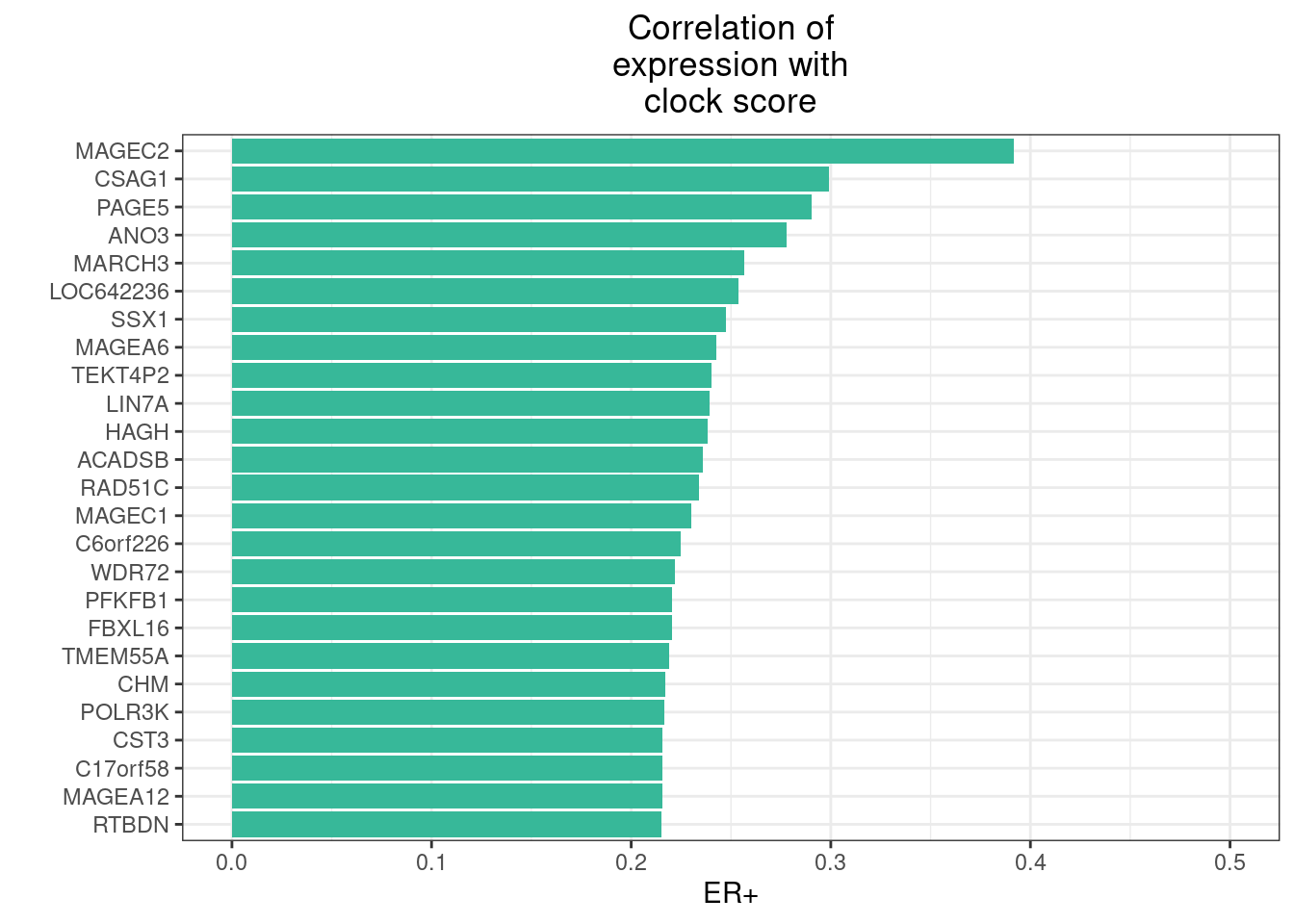    

5.6.0.2 Extended Data Figure 5b

gene_feat_df <- get_gene_features_df(c("MAGEC2", "PAGE5")) %>% filter(!is.na(clock))

options(repr.plot.width = 7, repr.plot.height = 4)
p_mage_page <- gene_feat_df %>%         
        filter(ER != "normal") %>% 
        mutate(ER = factor(ER, levels=c("ER+", "ER-"))) %>% 
        ggplot(aes(x=clock, y=expr, color=ER)) + 
            geom_point(size=0.2) +             
            xlab("Clock") + 
            scale_color_manual(values=annot_colors$ER1) + 
            ylab("Gene expression") + 
            facet_wrap(ER~name, scales="free_y", nrow=1) +             
            theme(aspect.ratio = 1) + 
            guides(color="none")
p_mage_page + theme_bw() + theme(aspect.ratio = 1)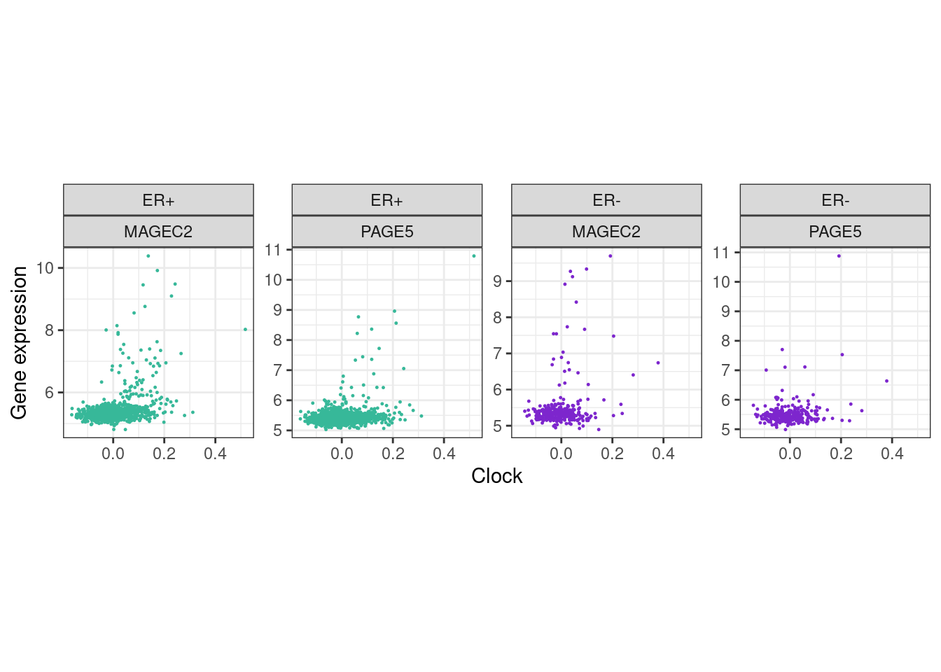

5.7 Plot score in different TOR regimes

all_mat_raw <- get_all_meth() %>% intervs_to_mat()

tor_strata <- loci_annot %>% mutate(tor_strata = cut(tor, breaks = main_config$genomic_regions$tor_low_mid_high, labels=c("late", "intermediate", "early"))) %>% pull(tor_strata) %>% forcats::fct_explicit_na()

samp_meth_tor <- tgs_matrix_tapply(t(all_mat_raw), tor_strata, mean, na.rm=TRUE) %>% t() %>% as.data.frame() %>% rownames_to_column("samp") %>% add_ER() %cache_df% here("data/samp_meth_tor.tsv") %>% as_tibble()

5.7.0.1 Extended Data Figure 4e

options(repr.plot.width = 9, repr.plot.height = 4)
p_early_late <- samp_meth_tor %>% 
    filter(ER != "normal") %>% 
    ggplot(aes(x=early, y=late, color=ER)) + 
        geom_abline(linetype = "dashed") + 
        geom_point(size=0.1) + 
        xlim(0.1, 0.9) + 
        ylim(0.1, 0.9) + 
        scale_color_manual(values=annot_colors$ER1) +         
        theme(aspect.ratio = 1) 

p_mid_early <- samp_meth_tor %>% 
    filter(ER != "normal") %>% 
    ggplot(aes(x=early, y=intermediate, color=ER)) + 
        geom_abline(linetype = "dashed") + 
        geom_point(size=0.1) + 
        xlim(0.1, 0.9) + 
        ylim(0.1, 0.9) + 
        scale_color_manual(values=annot_colors$ER1) +         
        theme(aspect.ratio = 1) 

samp_meth_tor %>% filter(ER != "normal") %>% summarise(cor_early_late = cor(early, late, method = "spearman", use = "pairwise.complete.obs"), cor_early_mid = cor(early, intermediate, method = "spearman", use = "pairwise.complete.obs"))

## # A tibble: 1 x 2
##   cor_early_late cor_early_mid
## 1      0.5723737     0.7680809

(p_early_late + theme_bw() + theme(aspect.ratio = 1) ) + (p_mid_early + theme_bw() + theme(aspect.ratio = 1) )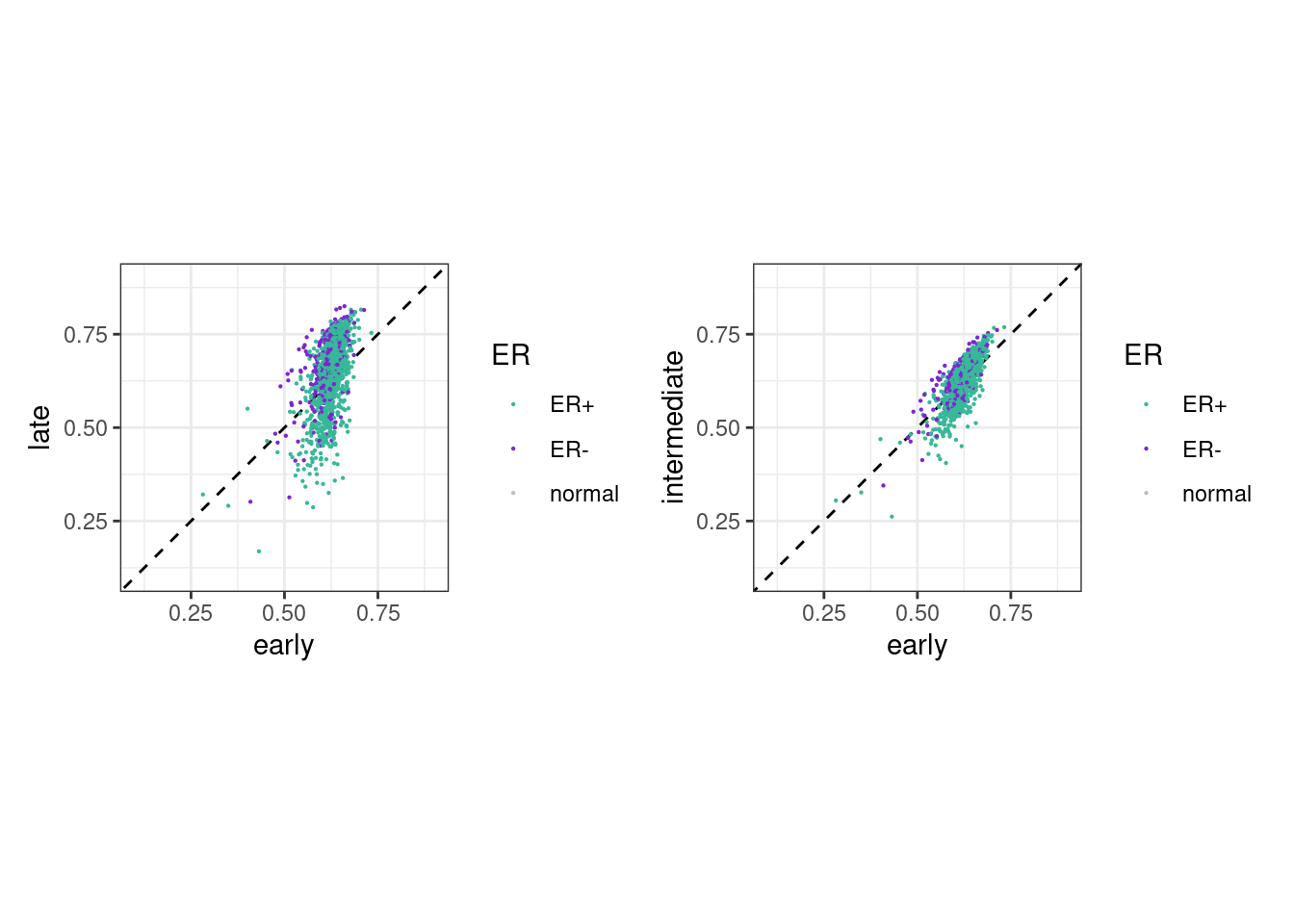

5.8 Plot High-Low clock tumors vs TOR

5.8.0.1 Extended Data Figure 4g

options(repr.plot.width = 4, repr.plot.height = 4)

df <- get_tor_clock_chrom_trace("chr1", "ER+", 1e5) %>% 
    filter(high_loss_n >= 50, low_loss_n >= 50) %>% 
    filter(!is.na(tor), !is.na(high_loss), !is.na(low_loss)) 

cor(-df$tor, df$high_loss - df$low_loss, method = "spearman")

## [1] -0.6187326

p_tor_high_low <- df %>%     
    ggplot(aes(x = -tor, y = high_loss - low_loss)) +
        geom_point(size=0.05, alpha=0.5) + 
        theme(aspect.ratio = 1) +
        ylim(-0.4, 0.025) + 
        xlab("Time of replication\n(Early -> Late)") +
        ylab("High Clock - Low Clock") 

p_tor_high_low + theme_bw() + theme(aspect.ratio = 1)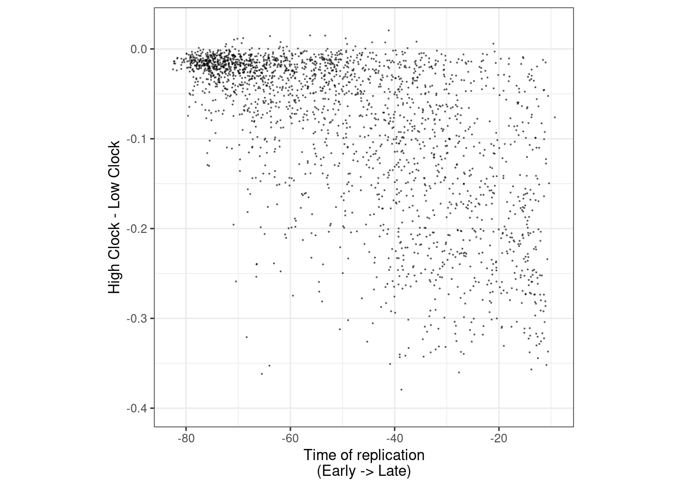

5.9 Plot correlation of loci to clock methylation

5.9.0.1 Extended Data Figure 4h

options(repr.plot.width = 8, repr.plot.height = 4)
p_loci_cor <- loci_annot %>% 
    left_join(get_all_summary_meth()) %>% 
    mutate(normal_meth = cut(normal, c(0,0.3,0.7,1), include.lowest=TRUE)) %>% 
    ggplot(aes(x=clock)) + 
    geom_density() + 
    facet_grid(.~normal_meth) + 
    ylab("Density") + 
    xlab("Correlation of loci to clock methylation")

## Joining, by = c("chrom", "start", "end")

p_loci_cor + theme_bw()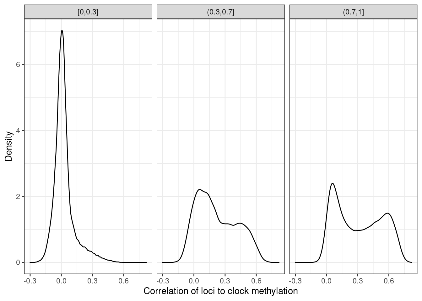

5.10 Plot distribution of methylation of clock in normal samples

normal_mat <- get_all_meth() %>% 
    select(chrom:end, any_of(normal_samples)) %>% 
    intervs_to_mat()
loci_annot_f <- loci_annot %>% 
    filter(cg_cont <= 0.02) %>% 
    mutate(tor = cut(tor, breaks=main_config$genomic_regions$tor_low_mid_high, labels=c("late", "mid", "early"), include.lowest=TRUE)) %>% mutate(tor = forcats::fct_explicit_na(tor)) %>% 
    intervs_to_mat()
normal_clock <- tgs_matrix_tapply(t(normal_mat[rownames(loci_annot_f), ]), loci_annot_f[, "tor"], mean, na.rm=TRUE) %>% 
    t() %>% 
    as.data.frame() %>% 
    rownames_to_column("samp") %>% 
    as_tibble() 
nrow(loci_annot_f)

## [1] 36420

5.10.0.1 Extended Data Figure 5b

options(repr.plot.width = 4, repr.plot.height = 4)
df <- normal_clock %>% 
    gather("tor", "meth", -samp) %>% 
    mutate(tor = factor(tor, levels = c("early", "mid", "late"))) %>%
    filter(!is.na(tor)) %>% 
    mutate(ER = "normal")

p_clock_normal <- df %>% 
        ggplot(aes(x = tor, y = meth, fill = ER)) +
        geom_boxplot(outlier.size=0.1, lwd = 0.5) +
        scale_fill_manual(values = annot_colors$ER1) +
        theme(aspect.ratio = 1) +
        guides(fill = FALSE) +
        xlab("Time of replication") +
        vertical_labs() +
        ylab("Methylation in normal samples\n(CpG content <= 2%)")

## Warning: `guides(<scale> = FALSE)` is deprecated. Please use `guides(<scale> =
## "none")` instead.

p_clock_normal + theme_bw() + theme(aspect.ratio = 1)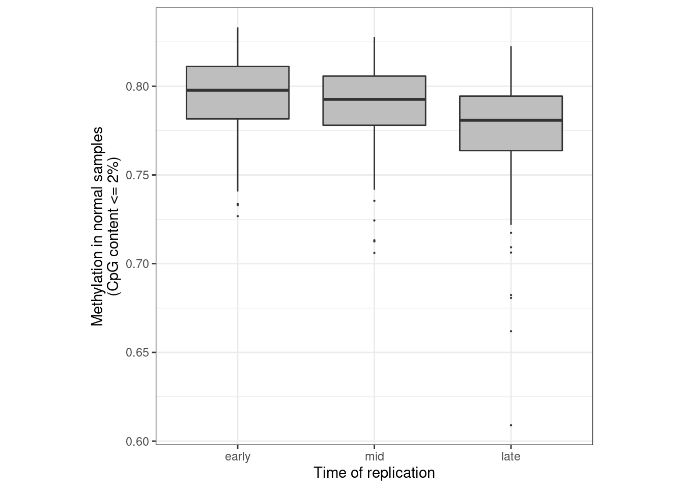

5.11 Compare clock layer to biological age

5.11.0.1 Extended Data Figure 5c

options(repr.plot.width = 12, repr.plot.height = 4)
df <- feats %>% 
    left_join(samp_data %>% select(samp, age)) 

## Joining, by = "samp"

df  %>% summarise(cor = cor(age, clock, method = "spearman", use = "pairwise.complete.obs"))

## # A tibble: 1 x 1
##          cor
## 1 0.06042711

p_age <- df %>% 
    ggplot(aes(x=age, y=clock, color=ER)) + 
        geom_point(size=0.5) + 
        scale_color_manual(values = annot_colors$ER1) + 
        theme(aspect.ratio = 1) + 
        xlab("Biological age") + 
        ylab("Clock") + 
        facet_grid(.~ER)

p_age + theme_bw() + theme(aspect.ratio = 1)

## Warning: Removed 30 rows containing missing values (geom_point).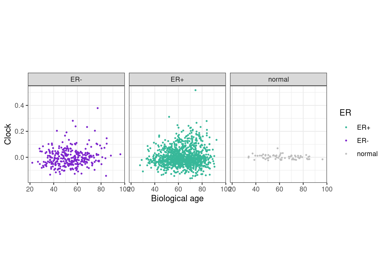

gc()

##             used   (Mb) gc trigger    (Mb)   max used    (Mb)
## Ncells   4907303  262.1    8028385   428.8    8028385   428.8
## Vcells 834169869 6364.3 1673781729 12770.0 1576695863 12029.3