2 METABRIC methylation data statistics

source(here::here("scripts/init.R"))

2.1 Breakdown of samples

2.1.0.1 Figure 1A

options(repr.plot.width = 7, repr.plot.height = 7)

p_donut <- samp_data %>%
        count(IHC) %>%
        filter(!is.na(IHC)) %>%
        left_join(
            tibble(
                IHC = c("ER+HER2-", "ER+HER2+", "ER-HER2+", "TNBC", "ADJNORMAL"),
                group = c("ER+", "ER+HER2+", "ER-HER2+", "Triple negative", "Adjacent normal")
            ), by = "IHC") %>%
        mutate(
            IHC = factor(IHC, levels = c("ER+HER2-", "ER+HER2+", "ER-HER2+", "TNBC", "ADJNORMAL")),
            lab = glue("{group}\n({n})")
        ) %>%
        ggpubr::ggdonutchart("n", "lab", fill = "IHC", lab.pos = "out", palette = annot_colors$IHC, font.family = "Arial", lab.font = c(6, "bold", "black"), ggtheme = ggpubr::theme_pubr(base_size = 6, base_family = "Arial")) + guides(fill = "none")


p_donut1 <- samp_data %>%
        count(ER1) %>%
        rename(ER = ER1) %>% 
        filter(!is.na(ER)) %>%
        left_join(
            tibble(
                ER = c("ER+", "ER-", "normal"),
                group = c("ER+", "ER-", "Adjacent normal")
            ), by = "ER") %>%
        mutate(
            ER = factor(ER, levels = c("ER+", "ER-", "normal")),
            lab = glue("{group}\n({n})")
        ) %>%
        ggpubr::ggdonutchart("n", "lab", fill = "ER", lab.pos = "out", palette = annot_colors$ER1, font.family = "Arial", lab.font = c(6, "bold", "black"), ggtheme = ggpubr::theme_pubr(base_size = 6, base_family = "Arial")) + guides(fill = "none")

p_donut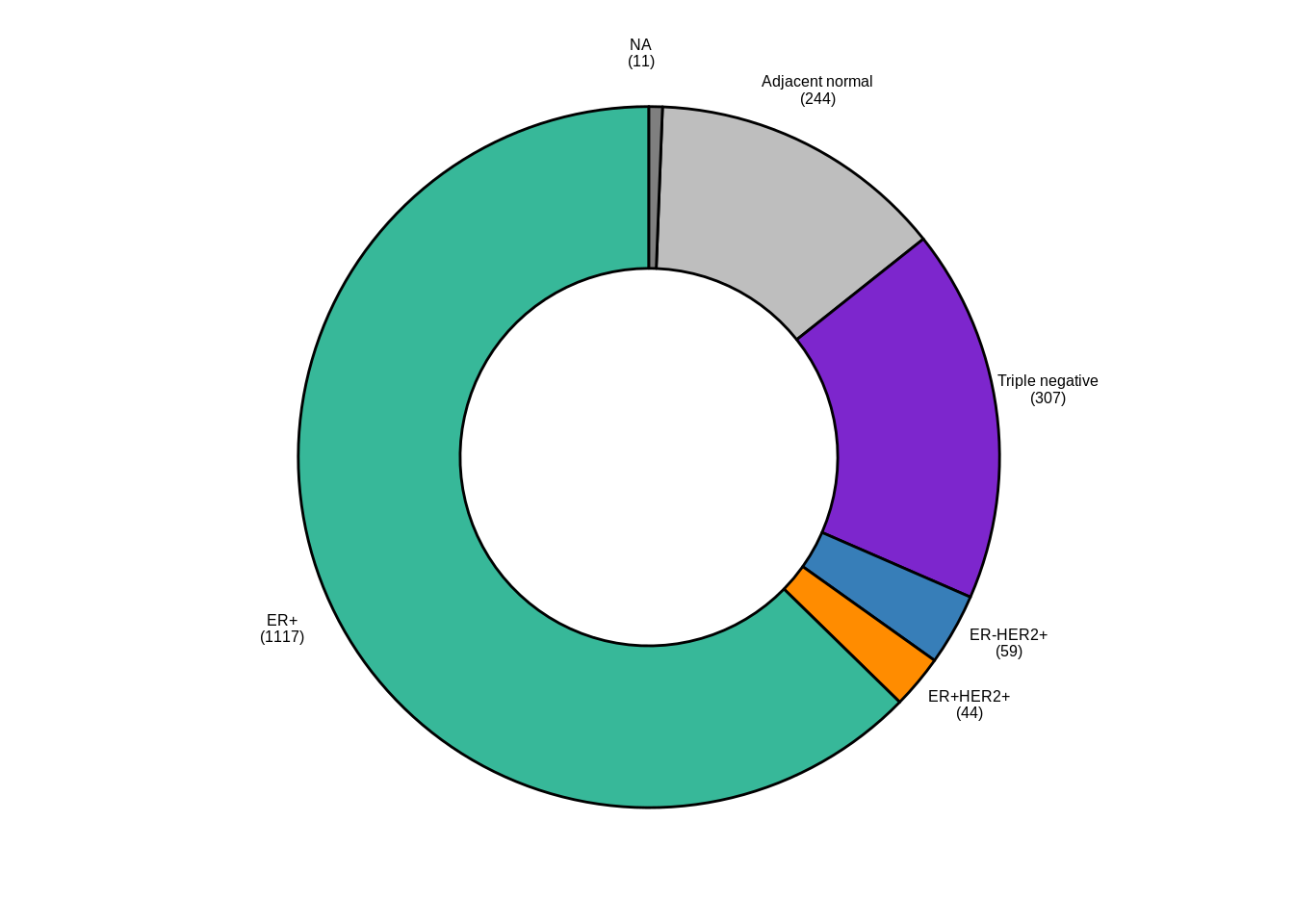

p_donut1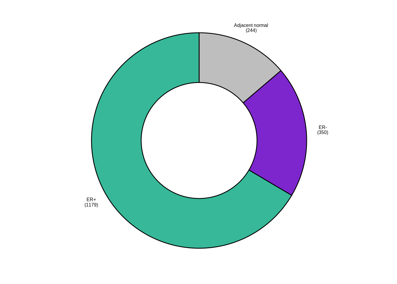

2.2 Number of samples

samp_data %>% mutate(ER1 = forcats::fct_explicit_na(ER1)) %>% count(ER1)

## # A tibble: 4 x 2
##         ER1    n
## 1       ER-  350
## 2       ER+ 1179
## 3    normal  244
## 4 (Missing)    9

2.3 Total number of reads

tot_reads <- fread(here("data/sample_qc.csv")) %>%     
    inner_join(samp_data %>% 
        select(track), by = "track") %>% 
    pull(total_reads) %>% 
    sum() 

glue("Overall, we used {round(tot_reads / 1e9, digits = 1)}B reads to cover {scales::comma(nrow(samp_data))} breast tumor and normal samples")

## Overall, we used 30.4B reads to cover 1,782 breast tumor and normal samples

2.4 Distribution of CpG coverage per sample

We calculate the distribution of every sample's CpG coverage:

samp_covs <- get_samples_coverage_dist(
    tracks = samp_data$track, 
    breaks = c(0:100, 1e5), 
    intervals = gintervals.all()) %cache_df% here("data/sample_coverage_dist.tsv") %>% as_tibble()

samp_covs <- samp_covs %>% left_join(samp_data %>% select(samp, ER = ER1), by = "samp")

2.4.0.1 Figure 1B

options(repr.plot.width = 7, repr.plot.height = 7)
p_comulative <- samp_covs %>%
        group_by(samp) %>%
        summarise(
            `>=10` = sum(cpgs[cov >= 10]),
            `>=20` = sum(cpgs[cov >= 20]),
            `>=30` = sum(cpgs[cov >= 30]),
            `>=50` = sum(cpgs[cov >= 50]),
            n_tot = sum(cpgs)
        ) %>%
        gather("type", "n", -samp, -n_tot) %>%
        ggplot(aes(x = n, color = type, y = 1 - ..y..)) +
        stat_ecdf() +
        scale_x_log10(labels = scales::scientific) +
        scale_color_viridis_d("CpG coverage") +
        scale_y_continuous(labels = function(x) round(x * length(unique(samp_covs$samp)))) +
        ylab("Samples with #CpGs >= x") +
        xlab("# of CpGs (log10)") +
        theme(aspect.ratio = 0.8)

p_comulative + theme_bw() + theme(aspect.ratio = 0.8)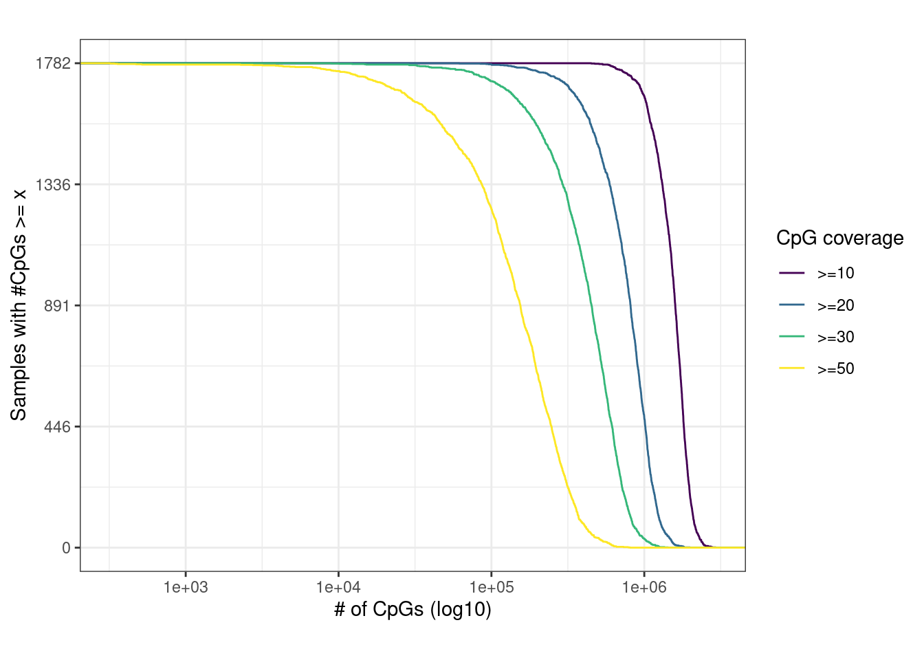

cov_above_10 <- samp_covs %>% 
    filter(cov >= 10) %>% 
    group_by(samp) %>% 
    summarise(cpgs = sum(cpgs))

df <- cov_above_10 %>%
    summarise(n_threshold = sum(cpgs >= 1e6), n_tot = n()) %>% 
    mutate(p = scales::percent(n_threshold / n_tot))

glue("Number of samples (Y axis) with a given number of CpGs (X axis) covered with at least 10, 20, 30 or 50 reads. For example, in all samples 449,710 CpGs are covered with over 10 reads.", n_cpgs = scales::comma(min(cov_above_10$cpgs)))

## Number of samples (Y axis) with a given number of CpGs (X axis) covered with at least 10, 20, 30 or 50 reads. For example, in all samples 449,710 CpGs are covered with over 10 reads.

glue("Using our version of the RRBS protocol {perc} of the samples were covered by more than 10 reads for more than 1M CpGs", perc = df$p)

## Using our version of the RRBS protocol 93% of the samples were covered by more than 10 reads for more than 1M CpGs

2.5 Distribution of covered CpGs

We screen for CpGs that are covered by at least 5 reads in half or more of the samples:

min_samples <- round(0.5 * nrow(samp_data))
min_samples

## [1] 891

cov_cpgs <- gscreen_coverage(samp_data$track, 5, min_samples) %>% annotate_loci() %cache_df% here("data/cov_cpgs.tsv") %>% as_tibble()

2.5.0.1 Figure 1C

options(repr.plot.width = 7, repr.plot.height = 3)
p_tss <- cov_cpgs %>%
        mutate(tss_d = abs(tss_d) + 1) %>%
        ggplot(aes(x = tss_d)) +
        geom_density() +
        scale_x_log10() +
        xlab("Distance from tss (bp)") +
        ylab("Density")

p_cg_cont <- cov_cpgs %>%
        ggplot(aes(x = cg_cont)) +
        geom_density() +
        xlab("CpG content (500 bp)") +
        ylab("Density")

(p_tss + theme_bw()) + (p_cg_cont + theme_bw())

## Warning: Removed 147 rows containing non-finite values (stat_density).

2.6 Promoter coverage

Distribution of mean promoter coverage over all METABRIC samples, considering 13,282 active promoters. Active promoters were defined as promoters that had log expression >7 in at least one of the METABRIC samples used in this paper.

2.6.0.1 Figure 1D

options(repr.plot.width = 4.6, repr.plot.height = 2.7)
prom_expr_cov <- get_promoter_expr_covs()

min_n_expr <- 0
max_expr <- 7

prom_expr_cov_active <- prom_expr_cov %>%
        filter(n_expr > min_n_expr, max_expr > !! max_expr)

p_prom_cov <- prom_expr_cov_active  %>%
        ggplot(aes(x = cov)) +
        geom_histogram(binwidth = 0.1) +
        scale_x_log10(breaks = c(1, 10, 50, 1000), labels = function(x) round(x)) +
        coord_cartesian(xlim = c(0.01,1500)) + 
        ylab("# of promoters") +
        xlab("Mean promoter coverage")

p_prom_cov + theme_bw()

## Warning: Transformation introduced infinite values in continuous x-axis

## Warning: Removed 119 rows containing non-finite values (stat_bin).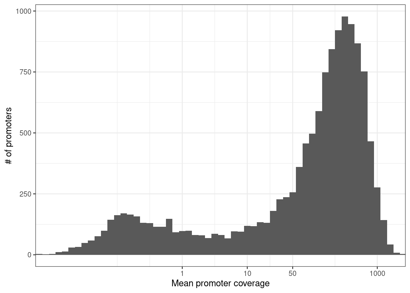

nrow(prom_expr_cov_active)

## [1] 13198

n_cov <- prom_expr_cov_active %>% filter(cov >= 20) %>% nrow()

glue("{perc} of the promoters were nevertheless covered with over 20 reads on average (mean coverage {cov}), facilitating quantitative analysis downstream.", perc = scales::percent(n_cov / nrow(prom_expr_cov_active)), cov = round(mean(prom_expr_cov_active$cov) ))

## 75% of the promoters were nevertheless covered with over 20 reads on average (mean coverage 246), facilitating quantitative analysis downstream.

samp_tot_calls <- get_sample_tot_meth_calls() %cache_df% here("data/sample_tot_meth_calls.tsv") %>% as_tibble()
samp_tot_calls_promoters <- get_sample_tot_meth_calls(promoter_intervs) %cache_df% here("data/sample_tot_meth_calls_promoters.tsv") %>% as_tibble()
tot_reads <- sum(samp_tot_calls$Sum)
tot_promoter_reads <- sum(samp_tot_calls_promoters$Sum)
glue("{perc} of the reads mapped to bona-fide promoters", perc = scales::percent(tot_promoter_reads / tot_reads))

## 9% of the reads mapped to bona-fide promoters

We can also calculate the % of MSP1 fragments that is covering a promoter:

well_covered_loci <- {
    msp1_meth <- get_msp1_meth()
    msp1_meth_f <- filter_avg_meth(msp1_meth$avg, normal_fraction = 0.7, tumor_fraction = 0.7)
    msp1_meth_f %>% select(chrom, start, end)
} %cache_df% here("data/well_covered_msp1_frags.tsv") %>% as_tibble()

n_loci <- nrow(well_covered_loci)
n_promoters <- well_covered_loci %>% gintervals.neighbors1(promoter_intervs) %>% filter(dist == 0) %>% nrow()

scales::percent(n_promoters / n_loci)

## [1] "10%"

2.7 Coverage per clinical annotations

samp_covs <- get_sample_tot_meth_calls() %cache_df% here("data/sample_tot_meth_calls.tsv") %>% as_tibble()
samp_covs <- samp_covs %>%
        select(samp, tot_cov = Sum) %>%
        left_join(samp_data %>% select(samp, stage, grade, iC10, ER = ER1), by = "samp") %>% 
        mutate(stage = ifelse(stage %in% c(0, "DCIS", 1), "0-1", stage)) %>% 
        mutate(stage = ifelse(ER == "normal", "N", stage)) %>% 
        mutate(grade = ifelse(ER == "normal", "N", grade)) %>% 
        mutate(stage = factor(stage, levels = c("N", "0-1", "2", "3", "4"))) %>% 
        mutate(grade = factor(grade, levels = c("N", "1", "2", "3")))        

2.7.0.1 Extended Data Figure 1a

options(repr.plot.width = 10, repr.plot.height = 3)
p_stage <- samp_covs %>%        
        filter(!is.na(stage), !is.na(ER)) %>%        
        arrange(stage, tot_cov) %>%
        mutate(samp = forcats::fct_inorder(samp)) %>%
        ggplot(aes(x = samp, y = tot_cov, fill = stage)) +
        geom_col() +
        theme(axis.ticks.x = element_blank(), axis.text.x = element_blank()) +
        scale_y_continuous(labels = scales::unit_format(unit = "M", scale = 1e-6)) +
        scale_x_discrete(breaks = FALSE) +
        scale_fill_manual(name = "Stage", values = c("N" = "gray", "0-1" = "black", "2" = "blue", "3" = "red", "4" = "orange")) + 
        xlab("") +
        ylab("# of methylation calls")

p_stage + theme_bw() + theme(axis.ticks.x = element_blank(), axis.text.x = element_blank())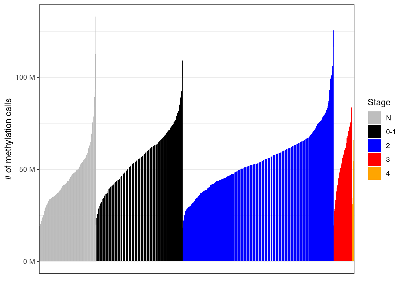

2.7.0.2 Extended Data Figure 1b

options(repr.plot.width = 10, repr.plot.height = 3)

p_iC10 <- samp_covs %>%
        filter(!is.na(iC10), !is.na(ER)) %>%
        mutate(iC10 = factor(iC10, levels = names(annot_colors$iC10))) %>%
        arrange(iC10, tot_cov) %>%
        mutate(samp = forcats::fct_inorder(samp)) %>%
        ggplot(aes(x = samp, y = tot_cov, fill = iC10)) +
        geom_col() +
        theme(axis.ticks.x = element_blank(), axis.text.x = element_blank()) +
        scale_y_continuous(labels = scales::unit_format(unit = "M", scale = 1e-6)) +
        scale_x_discrete(breaks = FALSE) +
        scale_fill_manual(values = annot_colors$iC10) +
        xlab("") +
        ylab("# of methylation calls")

p_iC10 + theme_bw() + theme(axis.ticks.x = element_blank(), axis.text.x = element_blank())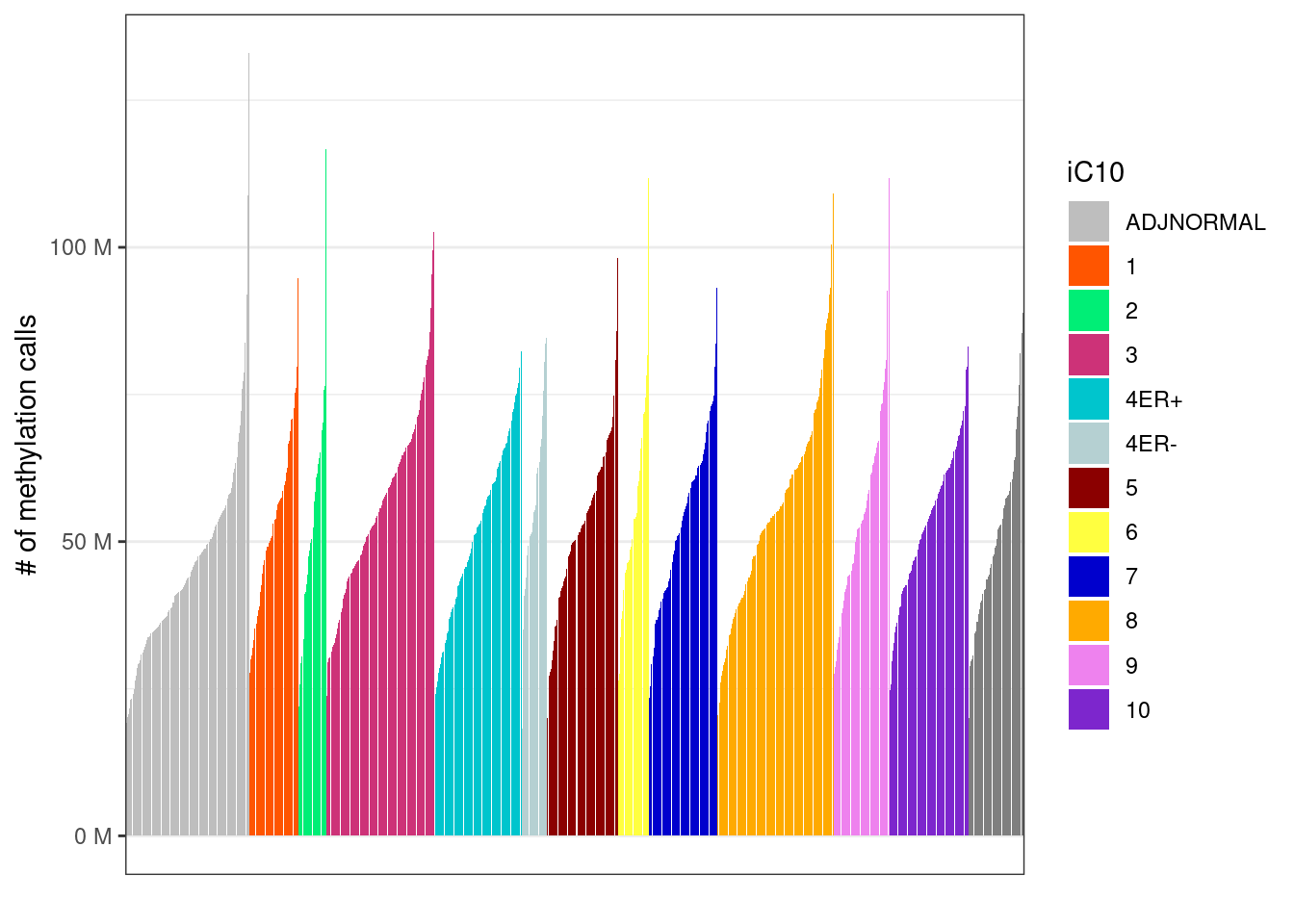

2.8 Marginal CpG coverage

cpg_mars <- covs_marginal(samp_data$track) %cache_df% here("data/cpg_cov_marginal.tsv") %>% as_tibble()

cpg_mars <- cpg_mars %>% mutate(mean_cov = cov / nrow(samp_data))
cov_cdf <- map_df(c(0:100, seq(200, 1000, 20)), ~ tibble(cov = .x, n = sum(cpg_mars$mean_cov >= .x)))  %cache_df% here("data/cpg_cov_cdf.tsv") %>% as_tibble()

2.8.0.1 Extended Data Figure 1b

options(repr.plot.width = 4.4, repr.plot.height = 3.5)

p_cov_cdf <- cov_cdf %>%
        filter(cov >= 1) %>%
        ggplot(aes(x = cov, y = n)) +
        geom_line() +
        scale_y_log10(labels = scales::scientific) +
        scale_x_log10() +
        xlab("Average CpG coverage") +
        ylab("# of CpGs")

p_cov_cdf + theme_bw() 

## Warning: Transformation introduced infinite values in continuous y-axis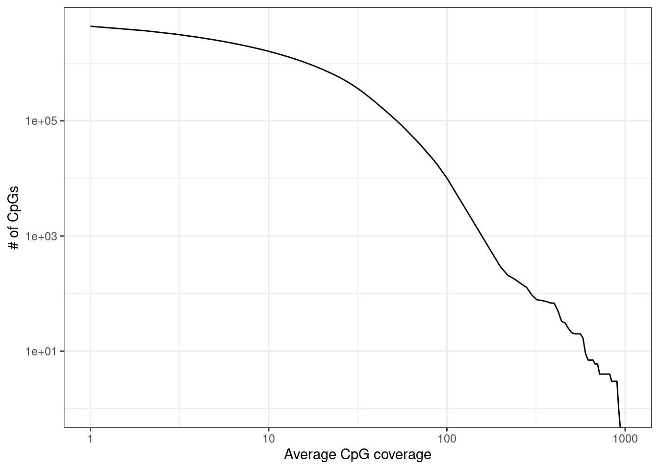

2.8.1 Marginal CpG coverage of k4me1 hotspots

conf <- main_config$genomic_regions$enhancers

conf$H3K4me1_tracks

## [1] "Roadmap.Breast_Luminal_Epithelial_Cells.H3K4me1"      
## [2] "Roadmap.Breast_Myoepithelial_Cells.H3K4me1_1"         
## [3] "Roadmap.Breast_Myoepithelial_Cells.H3K4me1_2"         
## [4] "encode.Tfbs.HMECwgEncodeBroadHistoneHmecH3k4me1StdSig"

conf$H3K4me1_thresh

## [1] 0.97

conf$H3K4me1_size

## [1] 200

intervs <- gpatterns.putative_enhancers(conf$H3K4me1_tracks, quant_thresh = conf$H3K4me1_thresh, normalize = conf$H3K4me1_size, min_tss_dist = conf$H3K4me1_tss_dist)
k4me1_mars <- cpg_mars %>%
    gintervals.neighbors1(intervs) %>%
    filter(dist == 0) %>%
    group_by(chrom1, start1, end1) %>%
    summarise(cov = sum(cov), mean_cov = cov / nrow(samp_data))
k4me1_mars <- k4me1_mars %>%
    ungroup() %>%
    select(chrom = chrom1, start = start1, end = end1, cov, mean_cov)

2.8.1.1 Extended Data Figure 1c

options(repr.plot.width = 4.4, repr.plot.height = 3.5)

p_k4me1 <- k4me1_mars %>%
        ggplot(aes(x = mean_cov, y = (1 - ..y..) * nrow(k4me1_mars))) +
        stat_ecdf() +
        scale_y_log10(labels = scales::scientific, breaks = c(10, 1e3, 1e4, 1e5)) +
        scale_x_log10(breaks = c(1, 10, 30, 100, 1000)) +
        xlab("Mean coverage") +
        ylab("# of k4me1 hotsplots") +
        vertical_labs()

p_k4me1 + theme_bw()

## Warning: Transformation introduced infinite values in continuous y-axis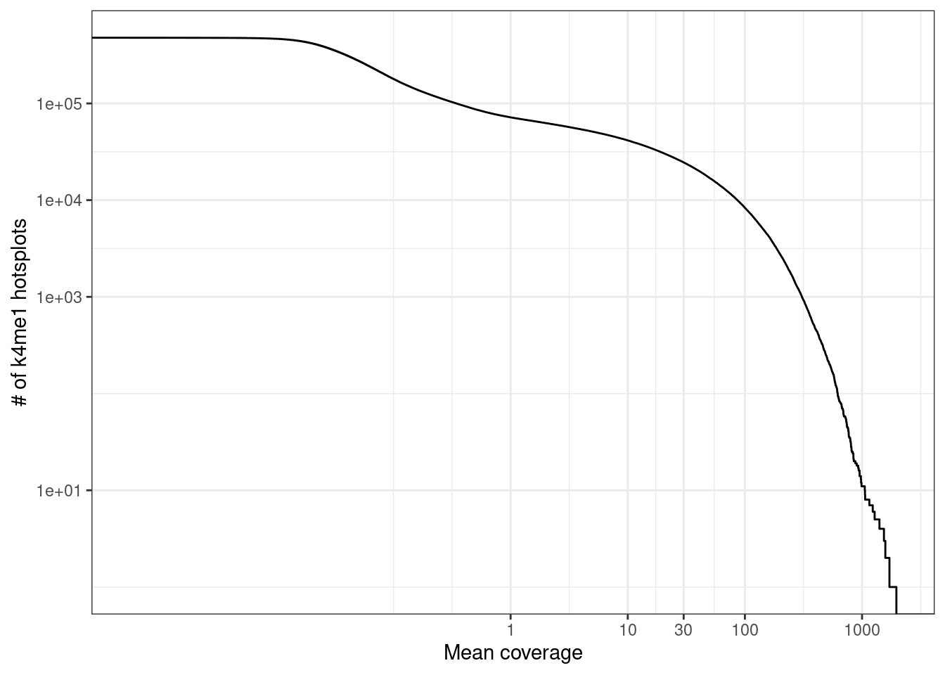

k4me1_mars <- cpg_mars %>%
    gintervals.neighbors1(enh_intervs_tumors) %>%
    filter(dist == 0) %>%
    group_by(chrom1, start1, end1) %>%
    summarise(cov = sum(cov), mean_cov = cov / nrow(samp_data))
k4me1_mars <- k4me1_mars %>%
    ungroup() %>%
    select(chrom = chrom1, start = start1, end = end1, cov, mean_cov)

options(repr.plot.width = 4.4, repr.plot.height = 3.5)

p_k4me1_tumors <- k4me1_mars %>%
        ggplot(aes(x = mean_cov, y = (1 - ..y..) * nrow(k4me1_mars))) +
        stat_ecdf() +
        scale_y_log10(labels = scales::scientific, breaks = c(10, 1e3, 1e4, 1e5)) +
        scale_x_log10(breaks = c(1, 10, 30, 100, 1000)) +
        xlab("Mean coverage") +
        ylab("# of k4me1 hotsplots") +
        vertical_labs()

p_k4me1_tumors + theme_bw()

## Warning: Transformation introduced infinite values in continuous y-axis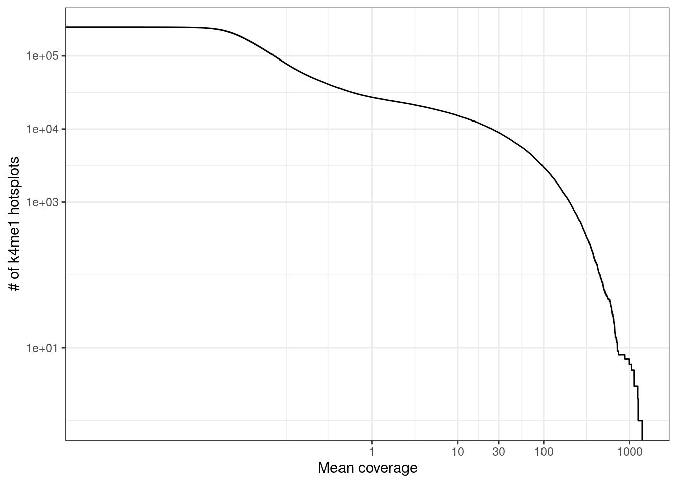

2.9 Sample cellularity

2.9.0.1 Extended Data Figure 1d

p_cellularity_cov <- samp_covs %>%
        filter(!is.na(ER)) %>%
        left_join(samp_data %>% select(samp, cna_cellularity)) %>%
        slice(sample(1:n())) %>%
        filter(ER != "normal") %>% 
        ggplot(aes(x = tot_cov, y = cna_cellularity, color = ER)) + 
            geom_point(size=0.1) + 
            scale_color_manual(values = annot_colors$ER1) + 
            scale_x_log10() + 
            theme(aspect.ratio = 1) + 
            guides(color = FALSE) + 
            xlab("Sample Coverage") + 
            ylab("Cellularity") + 
            vertical_labs() + 
            facet_grid(.~ER)

## Joining, by = "samp"

## Warning: `guides(<scale> = FALSE)` is deprecated. Please use `guides(<scale> =
## "none")` instead.

p_cellularity_cov

## Warning: Removed 279 rows containing missing values (geom_point).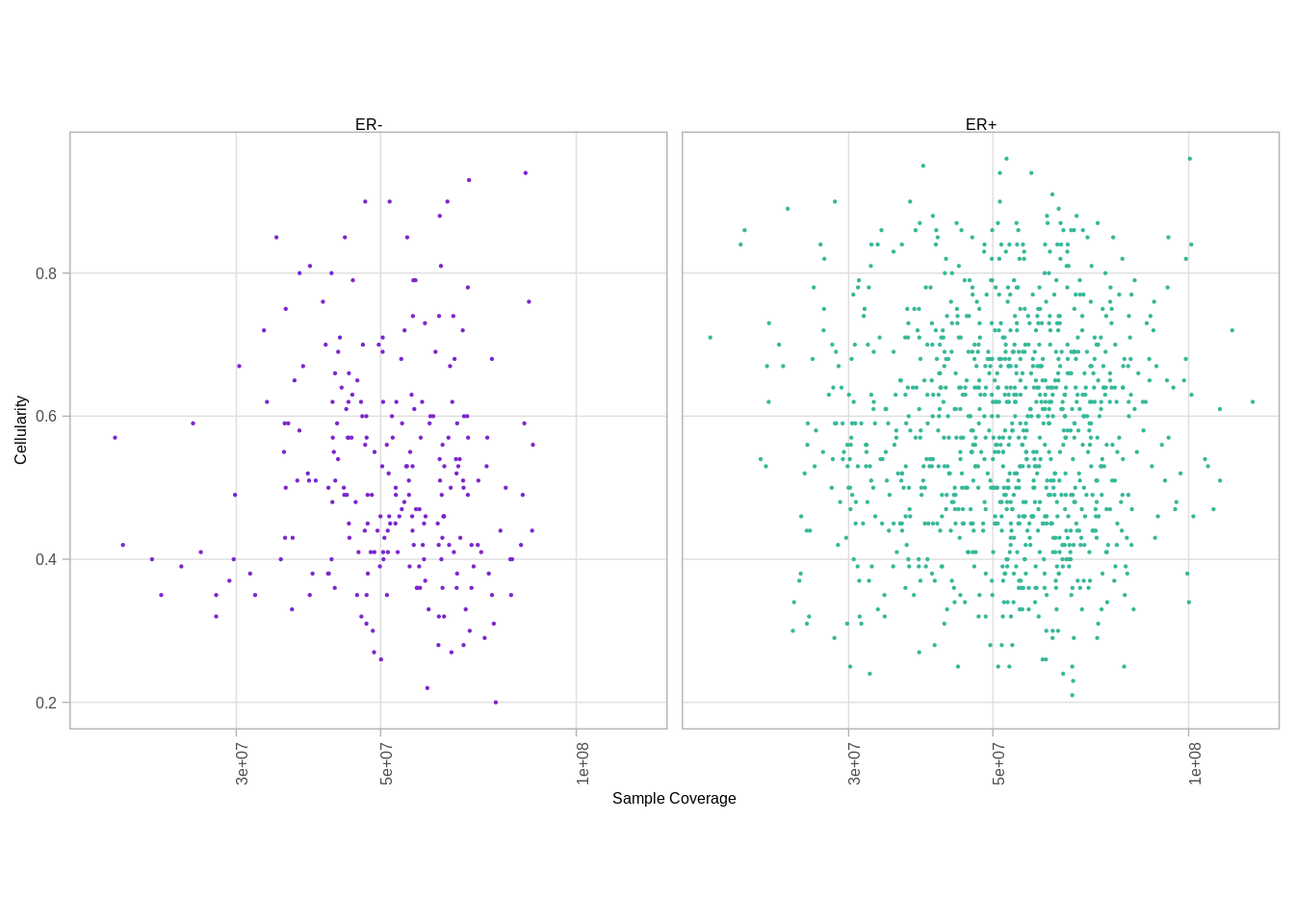

samp_genomic_meth <- get_genomic_avg_meth() %>% intervs_to_mat() %>% colMeans(na.rm=TRUE) %>% enframe("samp", "meth") %cache_df% here("data/samp_genomic_meth.tsv") %>% as_tibble()

p_cellularity_meth <- samp_genomic_meth %>%
        left_join(samp_data %>% select(samp, cna_cellularity, ER = ER1)) %>%
        filter(!is.na(ER)) %>%        
        slice(sample(1:n())) %>%
        filter(ER != "normal") %>% 
        ggplot(aes(x = meth, y = cna_cellularity, color = ER)) + 
        geom_point(size=0.1) + 
        scale_color_manual(values = annot_colors$ER1) + 
        theme(aspect.ratio = 1) + 
        guides(color = FALSE) + 
        xlab("Sample genomic methylation") + 
        ylab("Cellularity") + 
        facet_grid(.~ER)

## Joining, by = "samp"

## Warning: `guides(<scale> = FALSE)` is deprecated. Please use `guides(<scale> =
## "none")` instead.

p_cellularity_meth

## Warning: Removed 279 rows containing missing values (geom_point).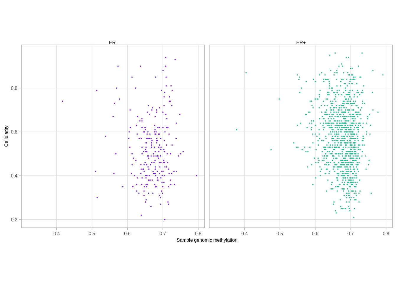

gc()

##             used   (Mb) gc trigger   (Mb)  max used   (Mb)
## Ncells   4497725  240.3    7606011  406.3   7606011  406.3
## Vcells 211991261 1617.4  562383716 4290.7 490804511 3744.6