Analyzing whole-organism scRNA-seq data with metacell

In this note we exemplify the application of metacell to a whole-organism scRNA-seq dataset, obtained using the MARS-seq protocol in the demosponge Amphimedon queenslandica (Sebe-Pedros et al. NEE 2018).

Initialize and load UMI matrix

library(metacell)

To start using metacell, we first need to initialize a database. This links the package to a directory (in this case aquedb) that stores all the objects:

if(!dir.exists("aquedb")) dir.create("aquedb/")
scdb_init("aquedb/", force_reinit=T)
#> initializing scdb to aquedb/

force_reinit=T instructs the system to override existing database objects. Otherwise, metacell reuses loaded objects to save time on reading and initializing them from the disk.

Next we load the UMI matrix to the system. In this case, we will import multiple MARS-seq batches and, for this, we also need to provide a table describing these experimental batches (to be downloaded).

download.file("http://www.wisdom.weizmann.ac.il/~arnau/metacell_data/Amphimedon_adult/MARS_Batches.txt","MARS_Batches.txt")
mcell_import_multi_mars("aque", "MARS_Batches.txt", base_dir="http://www.wisdom.weizmann.ac.il/~arnau/metacell_data/Amphimedon_adult/umi_tables")
#> will read AQFR0001
#> will read AQFR0002
#> will read AQFR0003
#> will read AQFR0004
#> will read AQFR0005
#> will read AQFR0006
#> will read AQFR0007
#> will read AQFR0008
#> will read AQFR0009
#> will read AQFR0010
#> will read AQFR0011
#> will read AQFR0012
#> will read AQFR0013
#> will read AQFR0014
#> will read AQFR0015
#> will read AQFR0016
#> will read AQFR0017
#> will read AQFR0018
#> will read AQFR0019
#> will read AQFR0020
#> will read AQFR0031
#> will read AQFR0032
#> will read AQFR0033
#> will read AQFR0034
#> will read AQFR0035
#> will read AQFR0036
#> [1] TRUE
mat = scdb_mat("aque")
print(dim(mat@mat))
#> [1] 49905  4992

The scdb_mat() command is returning a matrix object, which has one slot containing the count matrix (mat@mat), as well as additional features.

Before starting to analyze the data, we link the package to a figure directory:

if(!dir.exists("figs")) dir.create("figs/")
scfigs_init("figs/")

MetaCell uses a standardized naming scheme for the figures, to make it easier to archive and link analysis figures to the database objects. In principle, figures in the figures directory are named after the object data type they refer to (for example, mat for matrices, mc for metacells, and more, see below). The figure name then includes also the object name they refer to, and a suffix describing the actual figure type.

Exploring and filtering the UMI matrix

In MARS-seq we use ERCC standards, so we will first remove them from our UMI matrix. We start by identifying the ERCC gene IDs (rownames in the UMI matrix) and then we use a dedicated function to remove them from the original matrix and store a new matrix without them, under the name aque_noercc. We load this new matrix as our new mat object.

erccs <- rownames(mat@mat)[grepl("ERCC",rownames(mat@mat))]
mcell_mat_ignore_genes(new_mat_id="aque_noercc",mat_id="aque",ig_genes=erccs)
mat <- scdb_mat("aque_noercc")

To get a basic undersatnding of the new data, we will plot the distribution of umi count per cell:

mcell_plot_umis_per_cell("aque",min_umis_cutoff = 200)
#> [1] 200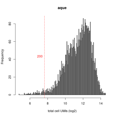

Umi distribution plot

As expected in a whole-organism dataset, we observe a very broad distribution of cell sizes (UMIs/cell). Before continuing we want to filter out very small cells (in this case <200 UMIs) and extremely large cells (in this case >12000 UMIs, which might represent doublets or FACS-sorting errors). Again, we store this new matrix (now with only filtered cells) under the name aque_filt. We can iteratively modify our filtering decisions given results of the downstream analysis.

cell_sizes <- colSums(as.matrix(mat@mat))
large_cells <- names(which(cell_sizes>12000))
small_cells <- names(which(cell_sizes<200))
mcell_mat_ignore_cells("aque_filt","aque_noercc",ig_cells=c(small_cells,large_cells))
mat <- scdb_mat("aque_filt")
print(dim(mat@mat))
#> [1] 49813  4743

Selecting gene markers

We will next select the marker genes for the downstream MetaCell analysis. First, we need to compute statistics on the distributions of each gene in the data, which is going to be our main tool for selecting informative markergenes.

mcell_add_gene_stat(gstat_id="aque", mat_id="aque_filt", force=T)
#> Calculating gene statistics...
#> will downsamp
#> done downsamp
#> will gen mat_n
#> done gen mat_n
#> done computing basic gstat, will compute trends
#> ..done

This generates a new object of type gstat under the name aque, by analyzing the count matrix with id aque_filt. We can explore interesting genes and their distributions (to do this, load the gene stats: gstats=scdb_gstat("aque")), or move directly to select a gene set for downstream analysis. For now, let's to the latter.

We create a new object of type gene set, called aque_feats, to which all potential gene markers that show a scaled size correlation below a certain threshold (T_szcor) are added. We can also use and combine other gene feature selection metrics such are downsampled varmean. But in the case of whole-organism datasets (with highly heterogeneous cell sizes, see above) this is not recommended. In addition, in this case we will also select genes based on third strategy (T_niche) that looks for genes with very restricted expression in a small group of cells. These genes are added to the list selected by size correlation.

We further refine our marker gene selection by asking (1) a minimum total of observed UMIs across the entire dataset (T_tot, >200 in this case) and (2) by also requiring selected genes to be detected in least three cells and with 3 or more UMIs in each of these cells (T_top3). Finally, we will exclude from our marker gene selection a list of genes (blacklist) that we defined as potentially problematic, such as ribosomal proteins. In general, it's a good a idea to only do this after initial analyses with all genes and then identifying these potentially problematic genes.

bl<- scan("http://www.wisdom.weizmann.ac.il/~arnau/metacell_data/Amphimedon_adult/bl_genes",what="")
mcell_gset_filter_multi(gset_id = "aque_feats",gstat_id="aque",T_tot=200,T_top3=2,T_szcor=-0.1,T_niche=0.08,force_new=T,blacklist=bl)
#> Selected 1006 markers

We can modify our parameters by plotting all genes and our selected gene set (shown in red). In this case, we plot the normalized size correlation statistic versus the mean expression of each gene:

mcell_plot_gstats(gstat_id="aque", gset_id="aque_feats")
#> agg_png 
#>       2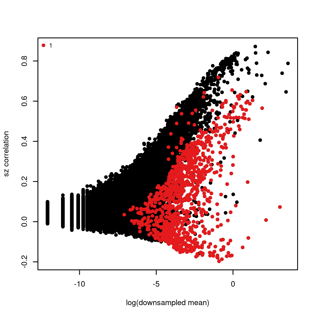

size correlation plot

Building the balanced cell graph

Assuming we are happy with the selected genes, we will move forward to create a similarity graph (cgraph), using a construction called balanced K-nn graph:

mcell_add_cgraph_from_mat_bknn(mat_id="aque_filt", 
                gset_id = "aque_feats", 
                graph_id="aque_graph",
                K=150,
                dsamp=F)
#> will build balanced knn graph on 4743 cells and 1006 genes, this can be a bit heavy for >20,000 cells
#> sim graph is missing 8 nodes, out of 4743

This adds to the database a new cell graph object named aque_graph. The K=100 parameter is important, as it defines the initial attempt of the system to assign neighbors for each cell and ultimately affects the size distribution of derived metacells. Note that constructing the graph can become computationally intensive if going beyond 20-30,000 cells.

Resampling and generating the co-clustering graph

The next step will use the cgraph to sample one thousand metacell partitions, each covering 75% of the cells and organizing them in dense subgraphs:

mcell_coclust_from_graph_resamp(
                coc_id="aque_coc1000", 
                graph_id="aque_graph",
                min_mc_size=20, 
                p_resamp=0.75, n_resamp=1000)
#> running bootstrap to generate cocluster
#> done resampling

The typical size distribution of the resampled metacells will be largely determined by the K parameter used for computing the cgraph. The resampling process may take a while if the graphs are very large. You can modify n_resamp to generate fewer resamples.

The resampling procedures creates a new coclust object in the database, named aque_coc1000, and storesthe number of times each pair of cells end up being part of the same metacells. The co-clustering statistics are used to generate a new similarity graph, based on which accurate calling of the final set of metacells is done:

mcell_mc_from_coclust_balanced(
                coc_id="aque_coc1000", 
                mat_id= "aque_filt",
                mc_id= "aque_mc", 
                K=20, min_mc_size=20, alpha=2)
#> filtered 1188359 left with 359944 based on co-cluster imbalance
#> building metacell object, #mc 45
#> add batch counts
#> compute footprints
#> compute absolute ps
#> compute coverage ps
#> reordering metacells by hclust and most variable two markers
#> reorder on Aqu2.1.42789_001 vs Aqu2.1.33784_001

We created a metacell object aque_mc, based on analysis of the co-clustering graph. The paramaetr K determine the number of neighbors we wish to minimally associate with each cell. alpha=2 is defining how harsh the filtering of co-cluster edges will be prior to running the metacell partition on them - e.g. alpha=2 will eliminate co-cluster relationships whenever one of the neighboring cells have K partners with more than twice as many co-cluster relationships. So the smaller the alpha, the harsher the filtering.

Removing outlier cells

We now have a preliminary metacell object. It is a good practice to make sure all metacells within it are homogeneous. This is done by the outlier scan procedure, which splits metacells whose underlying similarity structure supports the existence of multiple sub-clusters, and removes outlier cells that strongly deviate from their metacell?s expression profile.

mcell_plot_outlier_heatmap(mc_id="aque_mc", mat_id = "aque_filt", T_lfc=3)
#> agg_png 
#>       2
mcell_mc_split_filt(new_mc_id="aque_mc_f", 
            mc_id="aque_mc", 
            mat_id="aque_filt",
            T_lfc=3, plot_mats=F)
#> starting split outliers
#> splitting metacell 12
#> splitting metacell 21
#> splitting metacell 24
#> add batch counts
#> compute footprints
#> compute absolute ps
#> compute coverage ps

The first command generates a heatmap summarizing the detected outlier behaviors. This is possible only for datasets with modest size. The second command generates a new MC object aque_mc_f that we will use in dowstream analyses.

outliers fig

Creating heatmaps of metacells and genes

We will first assign random colors to our clusters (these can later be modified with custom color definitions, e.g. based on cell type assignments).

mc_f<- scdb_mc("aque_mc_f")
mc_f@colors <- colorRampPalette(c("darkgray", "burlywood1", "chocolate4","orange", "red", "purple", "blue","darkgoldenrod3", "cyan"))(ncol(mc_f@mc_fp))
scdb_add_mc("aque_mc_f",mc_f)
mc_f <- scdb_mc("aque_mc_f")

The filtered metacell object aque_mc_f can now be visualized. In order to do this effectively, we usually go through one or two iterations of selecting informative marker genes. The package can select markers for you automatically - by simply looking for genes that are strongly enriched in any of the metacells:

mcell_gset_from_mc_markers(gset_id="aque_markers", mc_id="aque_mc_f")

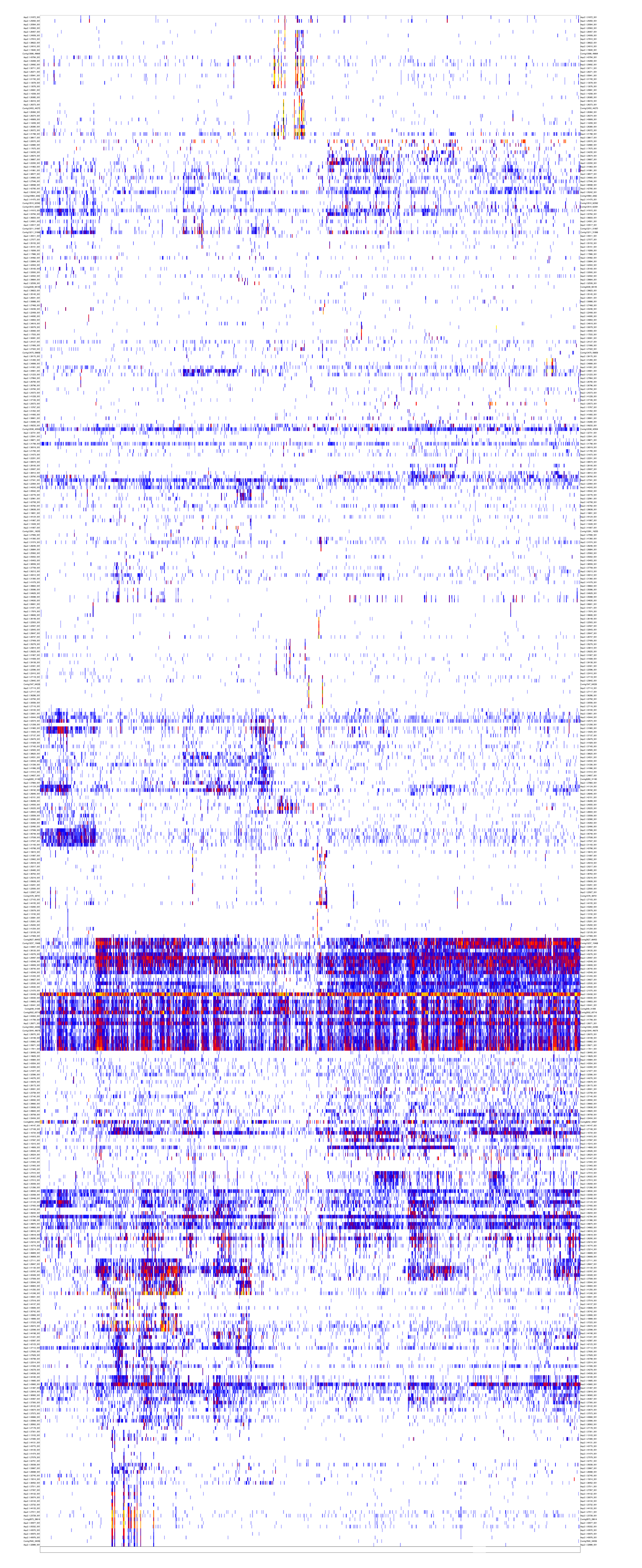
mcell_mc_plot_marks(mc_id="aque_mc_f", gset_id="aque_markers", mat_id="aque_filt",plot_cells = F)
#> setting fig h to 1000 md levels 0 num of marks 103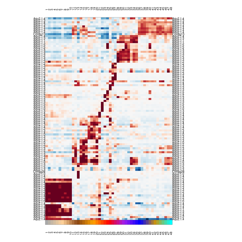

heatmap_marks

Note that the values plotted are color coded log2(fold enrichment) value of the metacell over the median of all other metacells. It can be useful to explore these values directly and visualize them in different ways - e.g.:

lfp <- log2(mc_f@mc_fp)
png("figs/example_barplot.png",h=400,w=1500);barplot(lfp["Aqu2.1.37150_001",],col=mc_f@colors,las=2,main="Cadherin",cex.main=3,cex.axis=1,ylab="log2FC",xlab="metacells");dev.off()
#> agg_png 
#>       2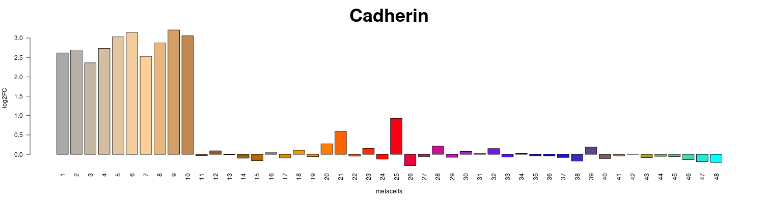

fold_enrichment_barplot

Projecting metacells and cells in 2D

Heat maps are useful but sometimes hard to interprets, and so we may want to visualize the similarity structure among metacells (or among cells within metacells). To this end we construct a 2D projection of the metacells, and use it to plot the metacells and key similarities between them (shown as connecting edges), as well as the cells. This plot will use the same metacell coloring we established before (and in case we improve the coloring based on additional analysis, the plot can be regenerated).

First we download the configuration file adapted to the Amphimedon dataset (parameters can be further modified and it is usually recommended to try different combinations:

download.file("http://www.wisdom.weizmann.ac.il/~arnau/metacell_data/Amphimedon_adult/config.yaml","config.yaml")

Now we override the default parameters, project the graph and plot the 2D projection:

tgconfig::override_params("config.yaml","metacell")
mcell_mc2d_force_knn(mc2d_id="aque_2dproj",mc_id="aque_mc_f", graph_id="aque_graph")
#> comp mc graph using the graph aque_graph and K 40
#> Missing coordinates in some cells that are not ourliers or ignored - check this out! (total 4 cells are missing, maybe you used the wrong graph object? first nodes WASP0001284WASP0002096WASP0002157WASP0018044
mcell_mc2d_plot(mc2d_id="aque_2dproj")
#> agg_png 
#>       2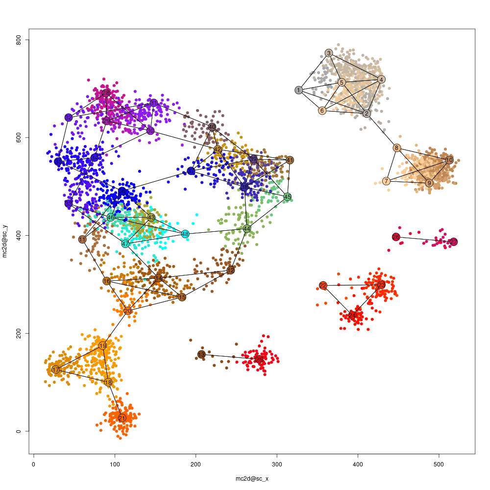

proj2d mean plot

Visualizing the metacell confusion matrix.

While 2D projections are popular and intuitive (albeit sometimes misleading) ways to visualize scRNA-seq results, we can also summarize the similarity structure among metacells using a "confusion matrix"" which encodes the pairwise similarities between all metacells. This matrix may capture hierarchical structures or other complex organizations among metacells.

We first create a hierarchical clustering of metacells, based on the number of similarity relations between their cells:

mc_hc <- mcell_mc_hclust_confu(mc_id="aque_mc_f", graph_id="aque_graph")

Next, we generate clusters of metacells based on this hierarchy, and visualize the confusion matrix and these clusters. The confusion matrix is shown at the bottom, and the top panel encodes the cluster hierarchy (subtrees in blue, sibling subtrees in gray):

mc_sup <- mcell_mc_hierarchy(mc_id="aque_mc_f",mc_hc=mc_hc, T_gap=0.04)

mcell_mc_plot_hierarchy(mc_id="aque_mc_f", 
                        graph_id="aque_graph", 
                        mc_order=mc_hc$order, 
                        sup_mc = mc_sup, 
                        width=2800, 
                        height=2000, 
                        min_nmc=2)
#> agg_png 
#>       2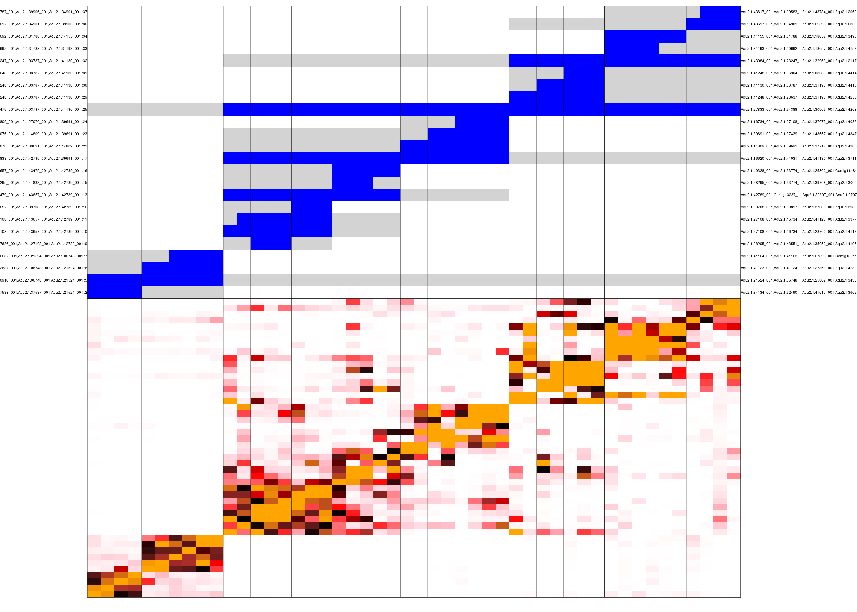

clustered confusion matrix

We can use this analysis to decide on the ordering and grouping of metacells, as well as to identify genes supporting different levels of this metacell hierarchy.

Arnau Sebe-Pedros

2021-12-21