Annotation of metacells

Introduction

This vignette demonstrates several ways to annotate metacells. It uses the genes relative enrichment of the metacells and the cross-metacell similarity matrix (confusion matrix) to identify metacells of a certain cell-type or cell state. The dataset used in this vignette is single-cell RNA-seq of T cells from lung cancer patients, from the Guo et al, Nat Med. 2018 paper.

Annotation of metacells is done by assigning a color to each metacell in the @colors vector in the metacell object. Information on the colors is stored in the @color_key data frame. It contains the columns 'group' (name of the type/state assigned to the metacell) and 'color', and might contain additional columns, depending on the method used to annotate the metacells, as will be shown below.

Setting up

The metacells partitioning we use here was generated from the transcript per million reads (TPM) input table Guo et al. supply. For more details see the guo2018.r script at Li_et_al_Cell_2018_Melanoma_scRNA code repository. We'll first download the input objects, specifically the unannotated metacell object. #{r, eval=TRUE, warning=FALSE} #download.file("http://www.wisdom.weizmann.ac.il/~lubling/metac_data/metacell_annotation/lung_db.tar.gz", destfile = #"lung_db.tar.gz") #system("tar xfz lung_db.tar.gz") #file.remove("lung_db.tar.gz") #

dir.create("lung_db", showWarnings = F)
for (f in c("cgraph.guo2018_tpm_scaled_filt_Tumor_Normal_Blood.Rda",
            "coclust.guo2018_tpm_scaled_filt_Tumor_Normal_Blood.Rda",
            "gset.guo2018_lateral.Rda",
            "gstat.guo2018_tpm_scaled_filt_Tumor_Normal_Blood.Rda",
            "lfp_screenshot.png",
            "mat.guo2018_tpm_scaled_filt_guo2018_lateral.Rda",
            "mat.guo2018_tpm_scaled_filt_Tumor_Normal_Blood.Rda",
            "mc.guo2018_tpm_scaled_filt_Tumor_Normal_Blood_outClean_nonAnn.Rda")) {
    download.file(paste0("https://schic2.s3.eu-west-1.amazonaws.com/metac_data/metacell_annotation/", f), destfile=paste0("lung_db/", f))
}

Now let's load the metacell package and define the output directories:

library(metacell)
library(dplyr)
#> 
#> Attaching package: 'dplyr'
#> The following objects are masked from 'package:stats':
#> 
#>     filter, lag
#> The following objects are masked from 'package:base':
#> 
#>     intersect, setdiff, setequal, union

scdb_init("lung_db", force_reinit=T)
#> initializing scdb to lung_db

dir.create("lung_figs", showWarnings = F)
scfigs_init("lung_figs")

For the sake of code clarity, lets define variables for the main metacell object IDs we'll soon use:

mc_non_ann_id   = "guo2018_tpm_scaled_filt_Tumor_Normal_Blood_outClean_nonAnn"
mc_id           = "guo2018_tpm_scaled_filt_Tumor_Normal_Blood_outClean"
graph_id        = "guo2018_tpm_scaled_filt_Tumor_Normal_Blood"
mat_id          = graph_id
lateral_gset_id = "guo2018_lateral"

Initial exploration of the metacells

It is often useful to start with semi-random coloring of metacells by assignment of sequentail colors to metacells. Since metacells are ordered by default, similar metacells will tend to have similar colors by this process. We'll first make a copy of the non-annotated input metacell object, in order not to overwrite it (we'll need it later on). Coloring is done by mc_colorize default function. The user can override the default color specturm used by supplying her own color spectrum (typically the output of colorRampPalette) to the spectrum parameter.

The function assigned colors in the @colors slot, yet the @color_key data frame is empty, since these colors are arbitrary and are not associated with any annotation.

mc_non_ann = scdb_mc(mc_non_ann_id)
scdb_add_mc(mc_id, mc_non_ann)

mc_colorize_default(mc_id)
mc = scdb_mc(mc_id)

print(mc@colors)
#>  [1] "#FFFFFF" "#F9F9F9" "#F3F3F3" "#EDEDED" "#E7E7E7" "#E1E1E1" "#DBDBDB"
#>  [8] "#D5D5D5" "#CFCFCF" "#CACACA" "#C4C4C4" "#BEBEBE" "#B9B9B9" "#B3B3B3"
#> [15] "#AEAEAE" "#AAA9A8" "#B5AFA6" "#C1B4A5" "#CCBAA3" "#D8C0A1" "#E4C59F"
#> [22] "#EFCB9D" "#FBD19B" "#F4C68E" "#E5B37C" "#D5A06A" "#C58D58" "#B67945"
#> [29] "#A66633" "#975321" "#8E4712" "#9E540F" "#AD610D" "#BD6E0A" "#CC7B08"
#> [36] "#DC8805" "#EB9503" "#FBA200" "#FF9300" "#FF7D00" "#FF6700" "#FF5100"
#> [43] "#FF3B00" "#FF2400" "#FF0E00" "#FA010A" "#ED052A" "#E10A4B" "#D40E6B"
#> [50] "#C7128B" "#BA16AB" "#AE1BCC" "#A11FEC" "#8C1CF1" "#7717F3" "#6113F5"
#> [57] "#4C0FF7" "#360AF9" "#2106FB" "#0B02FD" "#000FFF" "#0031FF" "#0053FF"
#> [64] "#0075FF" "#0098FF" "#00BAFF" "#00DCFF" "#00FFFF"
print(mc@color_key)
#> data frame with 0 columns and 0 rows

A concevenient way to explore the metacells is to generate a heatmap of gene enrichments on single cells or metacells. The input data is the genes relative footprint values across metacells over the median metacell footprint (the table under the @mc_fp slot). We'll usually use the log2 value of these ratios, and will term the matrix of log ratios lfp in this vignette.

We'll first select which genes to present with mcell_gset_from_mc_markers. Its basic usage expects an input metacell id (mc_id) and the name of the gene set to store the genes in (gset_id). This function screens for highly varying genes (max absolute lfp value above the config parameter scm_mc_mark_min_gene_fold, 1.5 by default) and selects the top N varying genes per metacell (N is defined in the scm_mc_mark_k_per_clust parameter, 5 by default). The union of the genes selected per metacell defines the output gene set.

mcell_gset_from_mc_markers(gset_id = mc_id, mc_id = mc_id)

Now we'll generate the heatmap, supplying the metacell id and the gene set id of the genes to show, and since we plot the cells (and not the metacells), also the mat id (from which the raw UMI counts are taken). The main configuration parameters that control the heatmap are mcp_heatmap_height and mcp_heatmap_width (figure height and width in pixels), mcp_heatmap_text_cex (text size, passed as cex param to text function) and mcp_heatmap_alt_side_text (logical, if true, plot odd gene names to the right and even to the left of the heatmap).

mcell_mc_plot_marks(mc_id = mc_id, gset_id = mc_id, mat_id = mat_id, plot_cells=T)
#> setting fig h to 1000 md levels 0 num of marks 86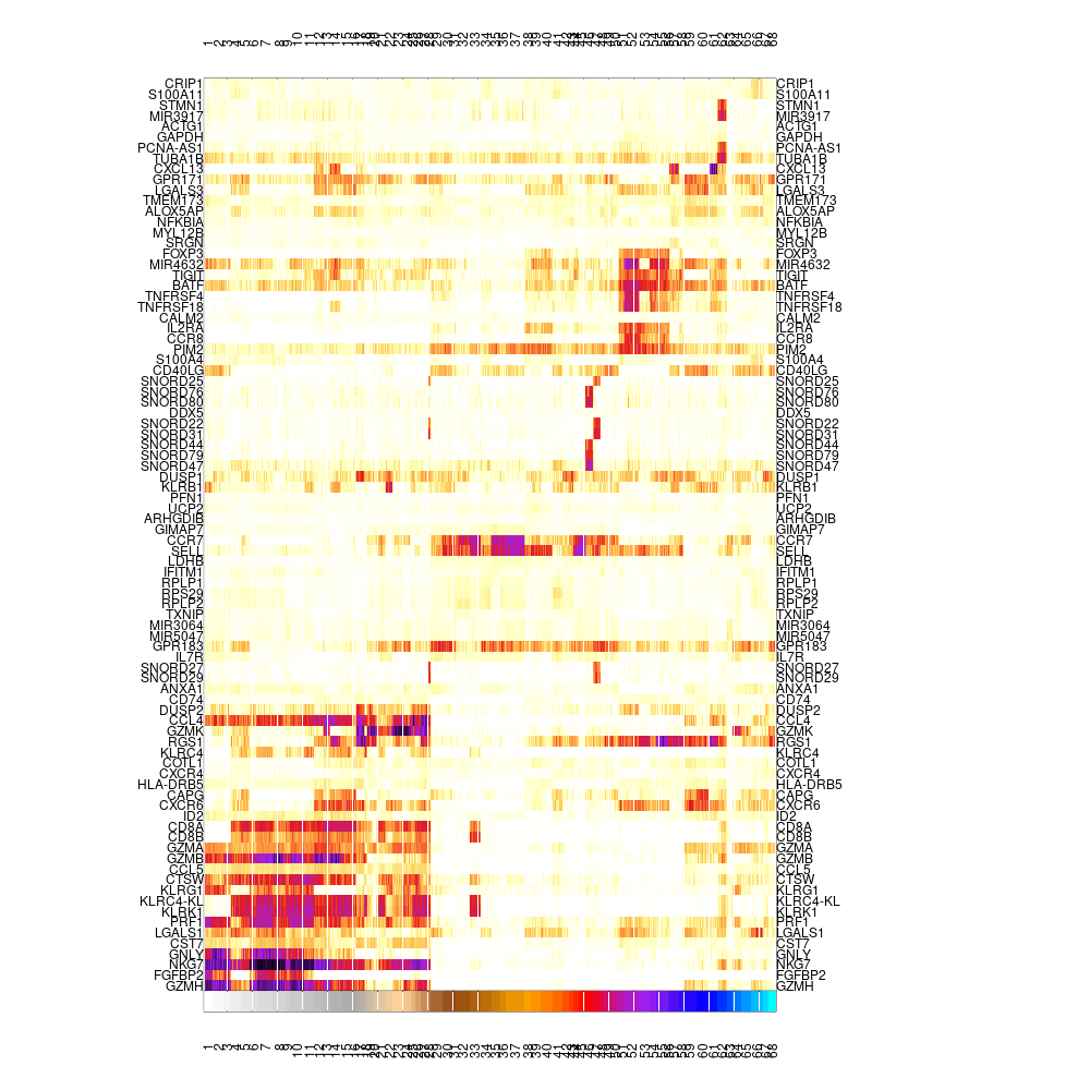

Varying genes footprint on single-cells, ordered by metacells

Lateral genes are enriched in several metacells regardless of the cell type or state. The obious example for such lateral gene program is cell cycle related genes. We often filter lateral genes from being features that affect the creation of metacells. When plotting gene-metacell heatmap, we can filter lateral genes from the displayed genes by supplying the lateral gene set id to the blacklist_gset_id parameter in mcell_gset_from_mc_markers. However, we might still want to see the expression of these genes across metacells in the heatmap, yet without letting them affect the ordering of metacells in the heatmap. To do so we generate 2 gene sets - both of highly variable genes across metacells, the first without and the second with only lateral genes. The first will be supplied to the gset_id param in mcell_mc_plot_marks and the second to the lateral_gset_id param. In this data, the lateral gene set contains cell cycle, IFNa response and stress related genes. The lateral genes are marked in red and are shown on at the top of the heatmap.

# prevent the lateral genes from being in the gene set
mcell_gset_from_mc_markers(gset_id = mc_id, mc_id = mc_id, blacklist_gset_id = lateral_gset_id)

# select variable genes from the lateral gene set
mcell_gset_from_mc_markers(gset_id = paste0(mc_id, "_lateral"), mc_id = mc_id, filt_gset_id = lateral_gset_id)
        
mcell_mc_plot_marks(mc_id = mc_id, gset_id = mc_id, mat_id = mat_id, fig_fn = scfigs_fn(mc_id, "cells_heat_marks_lat"), lateral_gset_id = paste0(mc_id, "_lateral"), plot_cells=T)
#> setting fig h to 1000 md levels 0 num of marks 76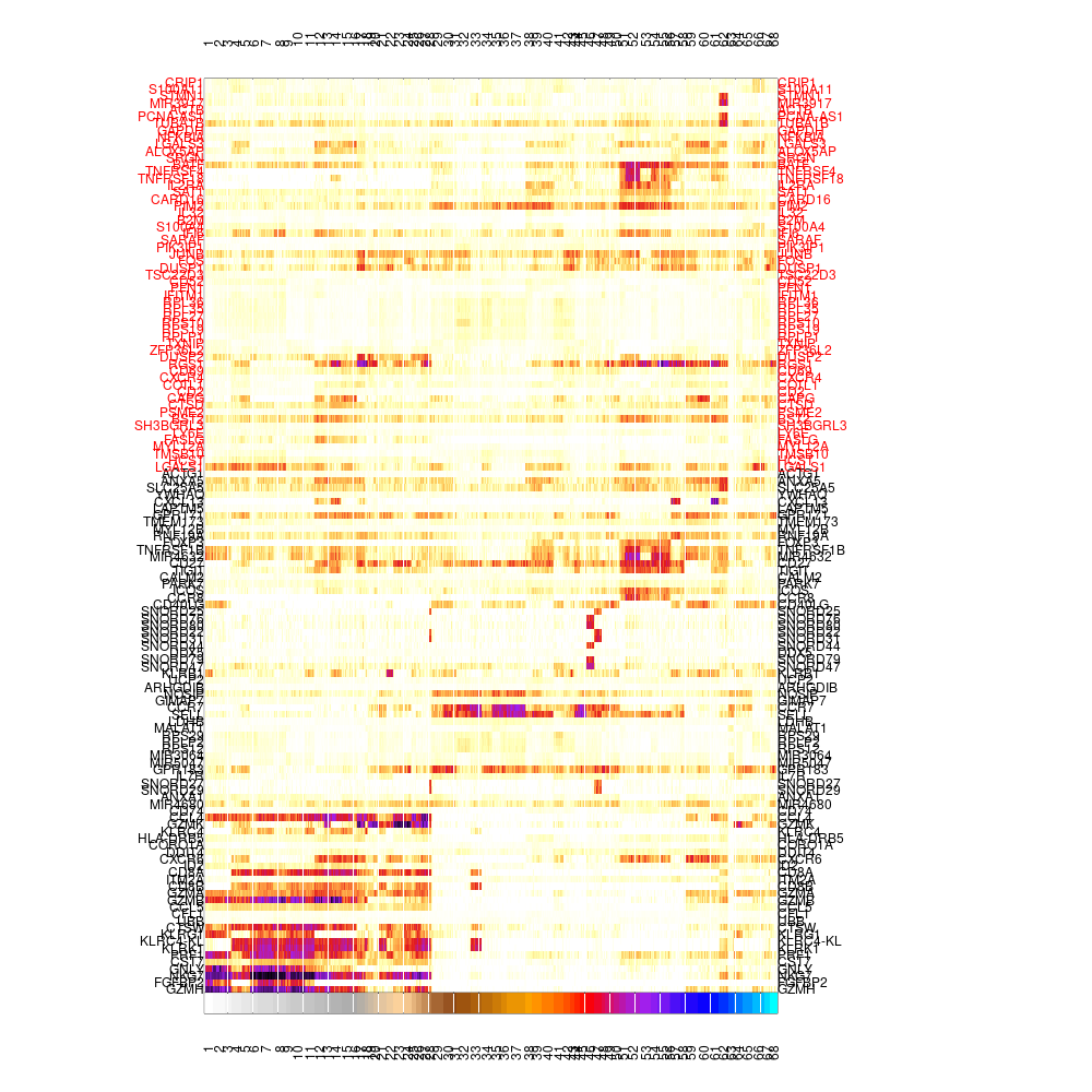

Varying genes footrprint on single-cells, ordered by metacells, lateral genes on top in red

Another quick and popular way to get a feeling on metacell similarity (and grouping) is to generate a 2D projection of cells and metacells, where the coordinates of each metacell and the edges between metacells are dictated by inter-metacell similarity. mcell_mc2d_force_knn builds the metacell 2D projection (mc2d object) and mcell_mc2d_plot generates the plot. The relevant configuration parameters affecting the plot are mcell_mc2d_height and mcell_mc2d_width (dimension in pixels), mcell_mc2d_plot_key (logical, whether to show the legend), mcell_mc2d_cex and mcell_mc2d_legend_cex (cells and legend size).

mcell_mc2d_force_knn(mc2d_id = mc_id, mc_id = mc_id, graph_id = graph_id)
#> comp mc graph using the graph guo2018_tpm_scaled_filt_Tumor_Normal_Blood and K 20
mcell_mc2d_plot(mc2d_id = mc_id, plot_edges = TRUE) 
#> agg_png 
#>       2

#> [1] TRUE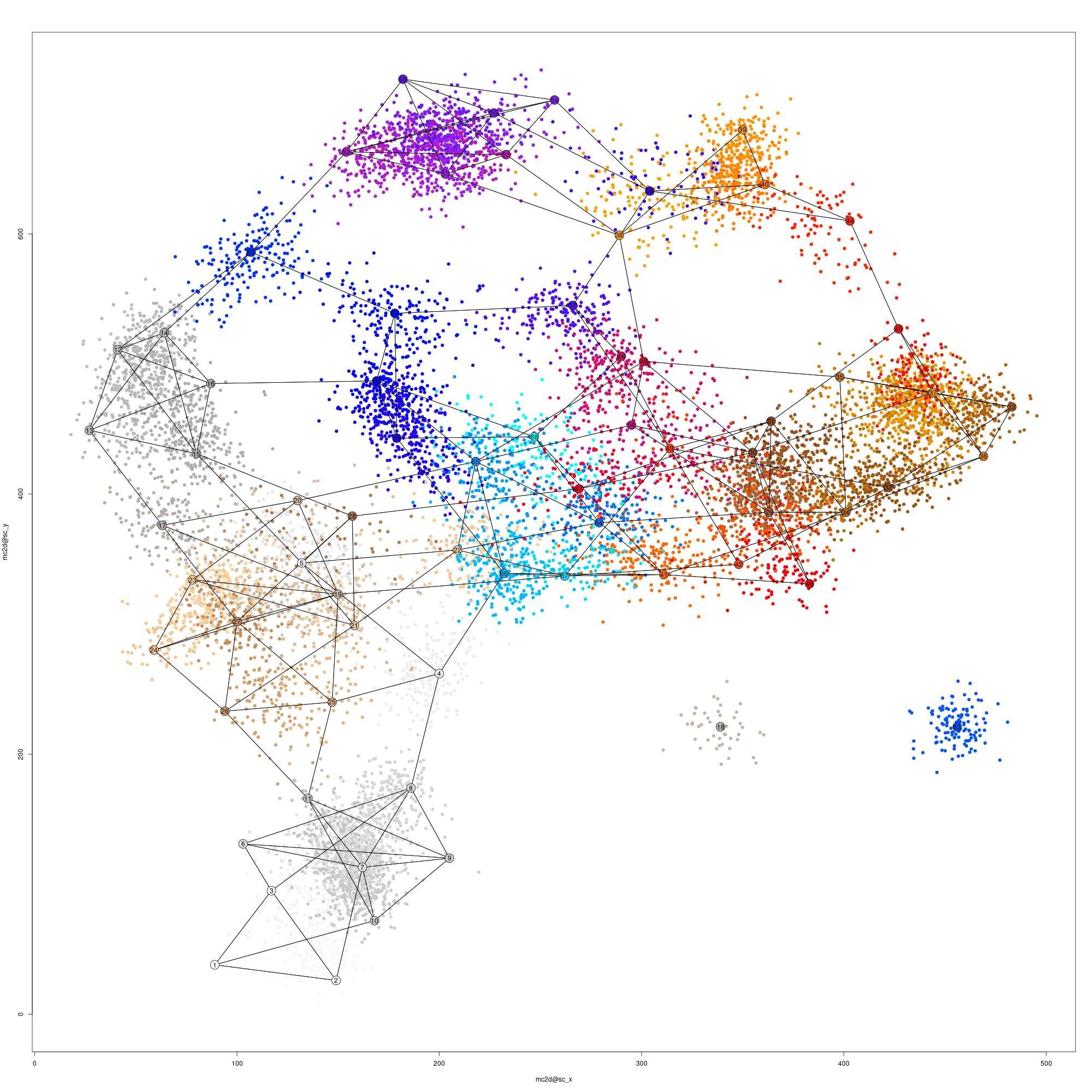

Single-cell and metacells 2D projection

Metacells gene enrichment table

As discussed above, the central way to characterize metacells is via the metacell gene enrichment table (termed here lfp, values in log2 ratio over median gene expression across metacells). We can generate a heatmap of the lfp, marking lateral genes in red and disabling them from affecting the metacells order (columns) as we did before when plotting a heatmap of genes and single-cells:

mcell_mc_plot_marks(mc_id = mc_id, gset_id = mc_id, mat_id = mat_id, fig_fn = scfigs_fn(mc_id, "mc_heat_marks_lat"), lateral_gset_id = paste0(mc_id, "_lateral"), plot_cells=F)
#> setting fig h to 1000 md levels 0 num of marks 76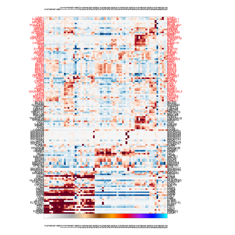

Varying genes footrprint on metacells, ordered by metecalls, blacklisted genes on top in red

It is also useful to do scatter plots for specific genes. In the example below, we're interested if the data contain Treg cells, so we plot CTLA4 vs CD4, and indeed there is a group of metacells enriched in both genes.

lfp = log2(mc@mc_fp)

plt = function(gene1, gene2, lfp, colors) 
{
    plot(lfp[gene1, ], lfp[gene2, ], pch=21, cex=3, bg=colors, xlab=gene1, ylab=gene2)
    text(lfp[gene1, ], lfp[gene2, ], colnames(lfp))
    
}
plt(gene1 = 'CD4', gene2 = 'CTLA4', lfp = lfp, colors = mc@colors)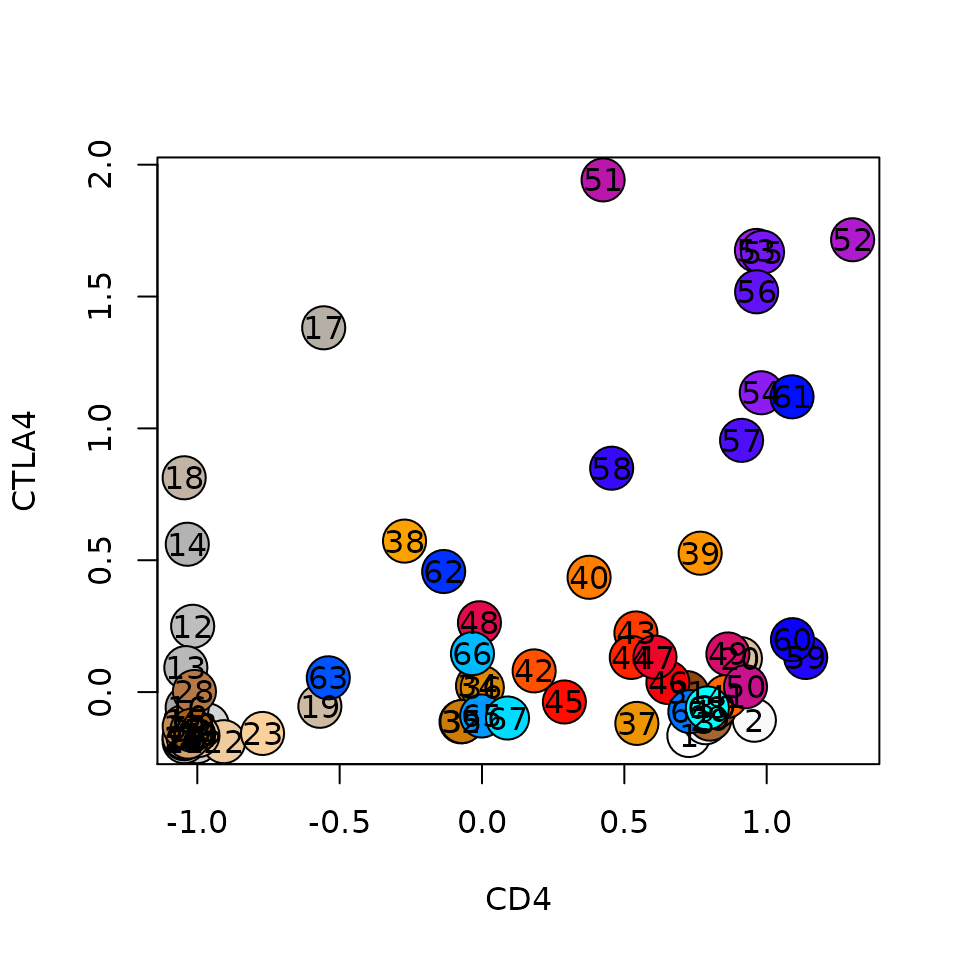

It is also useful to browse the lfp table itself. mcell_mc_export_tab exports the lfp table to a tab-delimited file. It filters genes with maximal lfp value above the T_fold parameter. The function reports the metacell size (n_cells) and mean UMIs per metacell (mean_umis), which is a proxy for the cell size. The group field contains the annotation of the metacell (this will be informative after the metacell coloring functions we'll present below). The metadata field names (columns in the mat object @cell_metadata table) can be supplied to the metadata_fields parameter. The function would then breakdown cells in each metacell on the values of the metadata field. Very useful to characterize the metacells if our data has informative metadata features.

mcell_mc_export_tab(mc_id = mc_id, gstat_id = mat_id, mat_id = mat_id, T_fold=2, metadata_fields=c('Patient', 'CD8_gate', 'Sex', 'Stage', 'Histology'))
lfp_tab = read.table(scfigs_fn(mc_id, "log2_mc_fp", ext = "txt"), header=F, sep="\t", stringsAsFactors = F)
knitr::kable(lfp_tab[1:40, 1:6])

V1	V2	V3	V4	V5	V6
Histology	adenocarcinoma	160.00	217.00	135.00	201.00
Histology	squamous cell carcinoma	7.00	27.00	2.00	5.00
Stage	I	137.00	193.00	37.00	14.00
Stage	III	27.00	48.00	99.00	192.00
Stage	IV	3.00	3.00	1.00	0.00
Sex	F	139.00	192.00	39.00	188.00
Sex	M	28.00	52.00	98.00	18.00
CD8_gate	-	166.00	243.00	129.00	1.00
CD8_gate	+	1.00	1.00	8.00	205.00
Patient	P0616A	13.00	10.00	15.00	0.00
Patient	P0616P	0.00	0.00	0.00	2.00
Patient	P0617	21.00	21.00	91.00	7.00
Patient	P0619	2.00	4.00	6.00	3.00
Patient	P0706	0.00	1.00	0.00	0.00
Patient	P0729	0.00	0.00	1.00	177.00
Patient	P0913	4.00	23.00	1.00	5.00
Patient	P1010	6.00	161.00	4.00	1.00
Patient	P1011	3.00	3.00	1.00	0.00
Patient	P1118	9.00	9.00	0.00	3.00
Patient	P1120	1.00	3.00	0.00	1.00
Patient	P1202	108.00	9.00	0.00	1.00
Patient	P1208	0.00	0.00	0.00	6.00
Patient	P1219	0.00	0.00	18.00	0.00
	mean_umis	19930.12	19913.84	19939.01	19951.63
	n_cells	167.00	244.00	137.00	206.00
	group	NA	NA	NA	NA
	mc_id	1.00	2.00	3.00	4.00
	TANK	-0.15	-0.12	-0.20	0.10
	LINC00892	0.50	0.47	0.36	0.19
	OST4	-0.56	0.26	0.25	0.30
	LINC00861	0.05	0.28	0.45	-0.32
	MIR1292	0.28	0.10	-0.03	-0.40
	MIR1282	-0.81	0.16	0.13	0.19
	PCNA-AS1	0.02	0.10	-0.22	-0.02
	ZEB2-AS1	0.91	0.70	1.00	0.05
	MIR1244-2	-0.13	-0.26	-0.70	0.07
	MIR3917	0.18	0.14	0.07	0.00
	MIR3656	0.21	0.07	-0.20	-0.01
	MIR3652	0.34	0.32	-0.34	-0.39
	MIR3615	1.19	0.83	1.14	-0.83

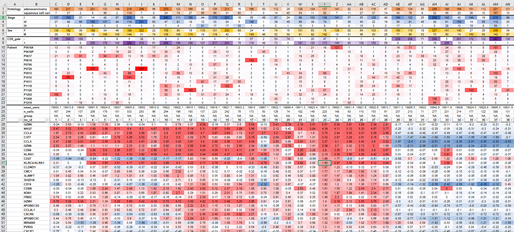
It is convenient to browse this table with MS Excel or a similar tool, and to color the gene's lfp values and the different metadata header rows (seperately, because of their different range), using the 'condistional formatting' options. The screenshot below shows a formatted lfp table. It is immediate to classify metacells as CD4 or CD8, to see patient specific metacells or pan-patient metacells etc. It is also useful to freeze the header rows and the gene names and then to sort the table content according to the metacell we're interseted in (in the screenshot below it's metacell #23), to quickly see its enriched genes. Since the metacells are clustered, it also makes the group of similar metacells pop-up very clearly.

Example of formatted lfp table

Manual annotation by thresholding gene enrichment

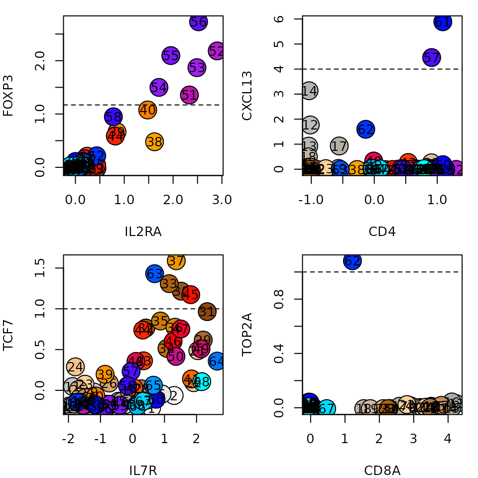
In many cases we'll have some prior knowledge on the cell types we expect to be represented by the metacells. Scatter plots of lfp values of selected genes can highlight these metacells. For instance, the plots below show metacells enriched in IL2RA and FOXP3, which are probably Tregs, CD4+ metacells that strongly express CXCL13, which probably represent Tfh cells, a single proliferating metacell enriched with TOP2A, and naive T cells, expressiong IL7R and TCF7. We can set a threshold on the lfp value of these genes (marked with dashed line) to assign an annotation to these metacells:

genes1 = c('IL2RA', 'CD4', 'IL7R', 'CD8A')
genes2 = c('FOXP3', 'CXCL13', 'TCF7', 'TOP2A')
cutoffs = log2(c(2.25, 16, 2, 2))
par(mfrow=c(2,2))
par(mar=c(4,4,1,1))
for (i in seq_along(genes1)) {
    plt(gene1 = genes1[i], gene2 = genes2[i], lfp = lfp, colors = mc@colors)
    abline(h=cutoffs[i], lty=2)
}

We define the annotations with their thresholds on genes in a tab-delimited file:

marks_colors = read.table(system.file("extdata", "guo2018_mc_partial_colorize.txt", package = "metacell"), sep="\t", h=T, stringsAsFactors=F)
knitr::kable(marks_colors)

group	gene	color	priority	T_fold
Treg	FOXP3	magenta	1	2.25
Tfh	CXCL13	darkolivegreen	1	16.00
Naive	TCF7	navajowhite2	1	2.00
Prolif	TOP2A	lightblue	1	2.00

The annotation name and its color are filled in the group and color columns. Threshold on each gene are in the T_fold column. Note that these are applied on the @mc_fp table, so should be fold change and not log2 fold-change. Each annotation can have several genes to define it, each with its own threshold. A metacell can match several rules, so the assigment might be ambigious. The priority value aims to address this. In the default mode, the lfp value of all genes passing their T_fold thresholds is multiplied by the gene priority and the gene with the maximal outcome is selected. If working in sequential coloring mode (setting configuration parameter mcp_colorize_by_seq_priority to be TRUE), genes are grouped by priority, and metacells are assigned to groups iteratively, starting with the genes in the first (smallest) priority, and only assigning groups to unassigned metacells in each iteration.

We use mc_colorize to annotate the metacelks with our gene rules, and plot the 2D projection to appreciate the result. Note that the @color_key table contains annotations, the plot has a legend. You can control its position with the legend_pos parameter (and control whether to show the legend at all with the logical configuration parameter mcell_mc2d_plot_key):

mc_colorize(new_mc_id = mc_id, mc_id = mc_non_ann_id, marker_colors=marks_colors)

mcell_mc2d_plot(mc2d_id = mc_id)
#> agg_png 
#>       2

#> [1] TRUE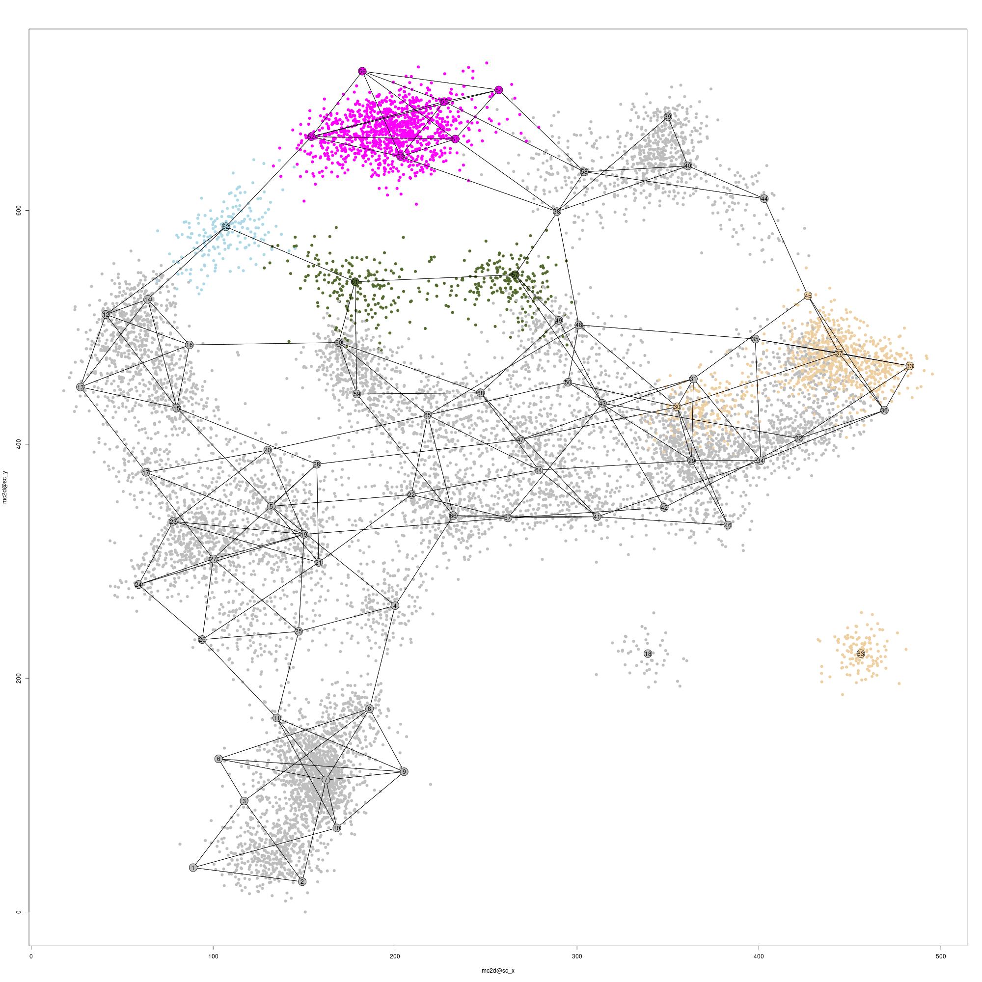

Single-cell and metacells 2D projection

Systematic annotation of metacells

A more comprehensive and systematic approach to annotate metacells uses the metacells 'confusion matrix', a metacell pairwise similarity matrix, summarizing the K-nn graph connectivity between all cells in each pair of metacells. We start by hierarchically clustering the metacells (columns) of the confusion matrix:

mc_hc = mcell_mc_hclust_confu(mc_id = mc_id, graph_id = graph_id)

Next, we generate clusters of metacells (super-metacells, or sup_mc for convenience) based on this hierarchy with mcell_mc_hierarchy. These clusters are nodes in the hierarchical tree of metacells that their branch length is longer then T_gap. We visualize the confusion matrix and these clusters with mcell_mc_plot_hierarchy. Only sup_mcs with more than min_nmc metacells in them are plotted. The confusion matrix is shown at the bottom, and the top panel encodes the cluster hierarchy by showing the subtree of each sup_mc in blue, and the sibling subtree in gray.

mc_sup = mcell_mc_hierarchy(mc_id = mc_id, mc_hc = mc_hc, T_gap = 0.04)

mcell_mc_plot_hierarchy(mc_id = mc_id, graph_id = graph_id, 
                        mc_order = mc_hc$order, 
                        sup_mc = mc_sup, 
                        width = 1200, height = 2400, 
                        min_nmc=2, show_mc_ids = T)
#> agg_png 
#>       2

#> [1] TRUE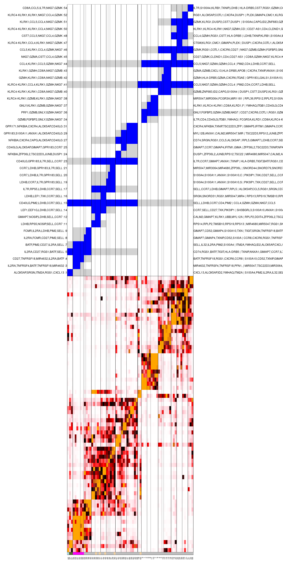

Clustered metacells confusion matrix

There are several lists of enriched genes for each subtree. Let's examine all the information supplied on a subree. For instance, subtree number 4 (which is clearly comprised of Treg metacells):

print(mc_sup[[4]])
#> $marks
#>    GAPDH CD27-AS1    CXCR6   CARD16     SELL    CTLA4 TNFRSF1B     ICOS 
#> 1.409033 1.425825 1.478982 1.527237 1.571408 1.609004 1.647381 1.729588 
#>  TNFRSF4    FOXP3     RGS1    TIGIT     CCR8     PIM2     SAT1     CD27 
#> 1.908381 1.955422 2.052494 2.065926 2.076183 2.108668 2.131010 2.170227 
#> TNFRSF18  MIR4632    IL2RA     BATF 
#> 2.185034 2.188458 2.318691 2.542111 
#> 
#> $min_marks
#>     CXCR6      SELL      CD82      RGS1     SIRPG      ICOS      IL32    CARD16 
#> 0.7418518 0.7487228 0.7501615 0.9337986 1.0267765 1.0475643 1.0644945 1.0738282 
#>     CTLA4      CD74      CCR8     GAPDH  CD27-AS1     FOXP3     TIGIT      SAT1 
#> 1.1351219 1.1766789 1.1937338 1.2025314 1.3105893 1.3563242 1.5938838 1.6433828 
#>     IL2RA      PIM2      CD27      BATF 
#> 1.7104313 1.7890192 2.0234116 2.1977205 
#> 
#> $marks_gap
#>      PKM     IFI6    IL1R2     ENO1     LDHA     SRGN     SAT1 TNFRSF1B 
#> 1.173707 1.179759 1.208043 1.212875 1.219272 1.235725 1.239677 1.257179 
#> APOBEC3C    GAPDH     ICOS     CTSC  MIR4632    DDIT4  TNFRSF4     CCR8 
#> 1.298520 1.340427 1.342362 1.389729 1.482165 1.484738 1.512940 1.667040 
#>    CXCR6     RGS1 TNFRSF18     BATF 
#> 1.860873 1.901821 1.971574 2.075978 
#> 
#> $marks_gap_anti
#>        GIMAP7        GIMAP4         TXNIP          CD52       S100A10 
#>    -2.1707354    -1.6104371    -1.5863388    -1.4286298    -1.1785400 
#>          FCMR GIMAP1-GIMAP5          SELL         LIME1       ALOX5AP 
#>    -1.1444732    -1.1084550    -1.0938374    -1.0360991    -0.9999712 
#>           AES          LDHB         GSTK1        RPL13A          CCR7 
#>    -0.9894325    -0.9848750    -0.9780960    -0.9670300    -0.9525264 
#>        GIMAP5          RPS6        UBXN11       RARRES3          LEF1 
#>    -0.9523882    -0.9315339    -0.8861049    -0.8690605    -0.8554596 
#> 
#> $mcs
#> [1] 55 53 52 51 54 56
#> 
#> $x_ord
#> [1] 6.5
#> 
#> $sup_mcs
#>  [1] 40 38 39 58 55 53 52 51 54 56

mcs - the ids of metacells in the subtree (those marked in blue)
sup_mcs - the ids of metacells in the subtree and in the sibling subtree (those marked in blue and gray)
x_ord - mean rank of the subtree metacells in the confusion matrix
marks - averaging lfp over mcs, showing the top 20 genes
min_marks - taking the minimal lfp value per gene over mcs, showing the top 20 genes
marks_gap - showing the genes with maximal difference between the average lfp over mcs and average lfp over metacells in the sibling subtree marks_gap_anti - similar to marks_gap but showing genes with minimal difference (e.g. enriched in the sibling subtree)

Top 5 marks genes are shown in the plot to the left of the sup_mc row, top 5 marks_gap are shown to the right, followed (after a 'pipe' sign) by the top 5 marks_gap_anti genes.

The annotation task based on this sup_mcs becomes the task of tagging sup-mcs, by browsing the figure and the more detailed sup_mc object, such that all metacells are covered by a tagged sup_mc. Annotation can also flow from bottom up, for instance, if we're insterseted in annotating CD8+ ZNF683+ enriched metacells: let's first see the lfp enrichment of both genes:

plt(gene1 = 'CD8A', gene2 = 'ZNF683', lfp = lfp, colors = mc@colors)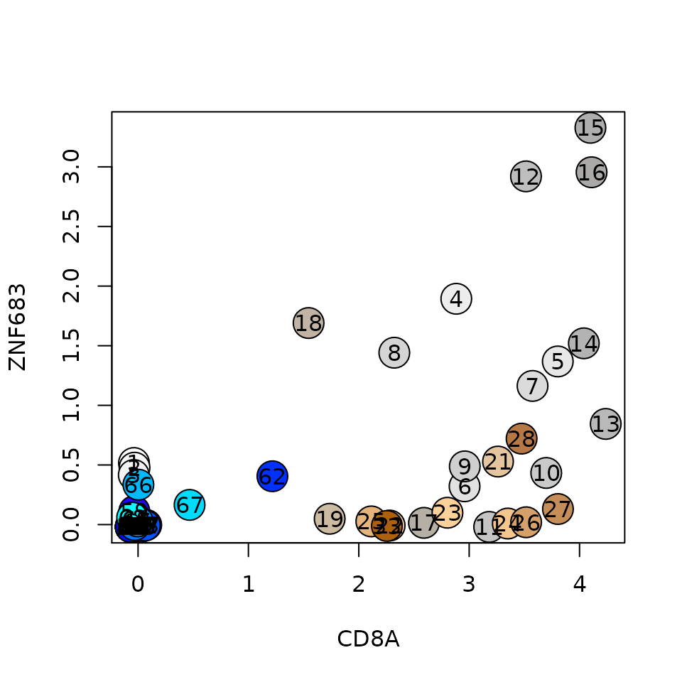

We see that there are 3 metacells with ZNF683 lfp values above 2.5, but where are these metacells within the sup_mc tree? We define here a simple helper function named query_sup_by_mcs, that gets a list of metacells and reports the sup_mcs that contain them (the id of the sup_mc, number of queried metacells, number of queried metacells inside the sup_mc and the sup_mc size). We usually aim to find the minimal sup_mc that contains most of the metacells we're interested in, in this case, sup_mc 42 seems like a reasonable choice:

query_sup_by_mcs = function(sup, mcs) 
{
    do.call('rbind', lapply(1:length(sup), function(i) { csup = sup[[i]]; data.frame(id=i, n_mcs=length(mcs), n_in=length(intersect(mcs, csup$mcs)), sup_size=length(csup$mcs)) })) %>% filter(n_in > 0) %>% arrange(sup_size)
}
query_sup_by_mcs(mc_sup, which(lfp['ZNF683', ] > 2.5))
#>   id n_mcs n_in sup_size
#> 1 43     3    2        4
#> 2 42     3    3        5
#> 3 40     3    3        7
#> 4 46     3    3       19
#> 5 44     3    3       28
#> 6 41     3    3       30

print(mc_sup[[42]])
#> $marks
#>        CAPG       COTL1    APOBEC3C        PRF1       ITGAE     ALOX5AP 
#>    1.741976    1.760421    1.774480    1.929533    2.148585    2.170378 
#>         ID2      ZNF683        CD8B       CXCR6        CTSW        GZMA 
#>    2.242233    2.313298    2.344979    2.444342    2.776128    2.842893 
#>        CCL5 KLRC4-KLRK1        CCL4        GZMH       KLRK1        CD8A 
#>    3.392455    3.481389    3.586614    3.655135    3.779911    3.999646 
#>        NKG7        GZMB 
#>    4.393001    4.595379 
#> 
#> $min_marks
#>       ITGAE        CTSD    APOBEC3C    APOBEC3G      GPR171         ID2 
#>    1.012721    1.021769    1.029850    1.127767    1.148459    1.183031 
#>       COTL1        PRF1        CCL4        GZMA        CTSW       CXCR6 
#>    1.206467    1.368101    1.731148    1.834879    1.891544    2.115394 
#>        CD8B        CCL5 KLRC4-KLRK1        GZMH        GZMB       KLRK1 
#>    2.122480    2.879629    3.070701    3.145283    3.369617    3.434703 
#>        CD8A        NKG7 
#>    3.514828    3.649621 
#> 
#> $marks_gap
#>     UCP2    SIRPG    ITM2A HLA-DRB1     IDH2   CXCL13    DDIT4      LCK 
#> 1.158478 1.168008 1.174318 1.197966 1.199905 1.203829 1.231473 1.268832 
#>   ARPC1B     GZMB     CD74   CORO1A APOBEC3C    COTL1 HLA-DRB6    ITGAE 
#> 1.271518 1.277664 1.306401 1.334704 1.435025 1.450852 1.586647 1.645951 
#>    CXCR6     GZMA HLA-DRB5     GZMH 
#> 1.681105 1.740864 1.799916 1.830240 
#> 
#> $marks_gap_anti
#>       IL7R      RPLP2    S100A10     LGALS1     GPR183     S100A4      RPS12 
#> -1.6705130 -1.4081441 -1.3791475 -1.2715754 -1.1557306 -1.0069529 -1.0064458 
#>      ANXA1      RPS14    S100A11      RPL35       GNLY      RPL36     TMSB10 
#> -0.9702105 -0.9231261 -0.9154989 -0.9065101 -0.9012424 -0.8934304 -0.8931744 
#>      RPL30      RPS16      RPS29      RPS10      RPL27      RPL32 
#> -0.8871693 -0.8416471 -0.8384013 -0.8373846 -0.8348400 -0.8348025 
#> 
#> $mcs
#> [1] 16 13 14 12 15
#> 
#> $x_ord
#> [1] 54
#> 
#> $sup_mcs
#> [1] 16 13 14 12 15  5  4

The list of annotated sup_mcs should be in a tab-delimited table containing the id of the sup_mc, its name and color, as shown below. Note that the order of entries matters - the annotation function process this table sequentially, so the newest entry overrides previous ones (if a metacell below to several sup_mcs in the table). It is actually useful in some cases, where you first define a large group of metacells and then pick from within it a smaller group and re-annotate it.

supmc_tab = read.table(system.file("extdata", "guo2018_supmc.txt", package = "metacell"), sep="\t", h=T, stringsAsFactors=F)
knitr::kable(supmc_tab)

supid	color	name
2	#107538	Tfh
4	#59b56f	tumor-Treg
8	#a3ffb9	blood-Treg
17	#b3d4f0	naive-TCF7
27	#6d8eaa	naive-CXCR6
34	#cee6b9	CD4-cyto
37	#fdb913	CD8-cyto
40	#a76eaf	CD8-dysf
51	#d29bc6	CD8-GZMK

Sometimes the sup_mcs will not cover all the metacells. Usually this is the case if we have rare cell types represented by a single metacell. For instance Mucosal associated invariant T cell (MAIT) cells in our data here:

plt(gene1 = 'SLC4A10', gene2 = 'KLRB1', lfp = lfp, colors = mc@colors)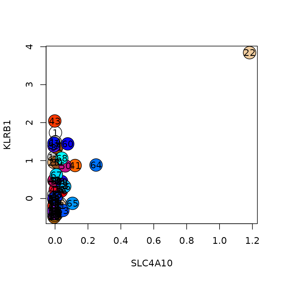

We can annotate these metacells by defining thresholds on genes. Note that the T_fold threshold in this case is compared to the log2 lfp value. Processing of this table is also sequetial, so if a metacell matches several rules, the last one overwrites any of the previous rules, and coloring by this table will also override any coloring done based on the sup_mcs table.

knitr::kable(read.table(system.file("extdata", "guo2018_marks.txt", package = "metacell"), sep="\t", h=T, stringsAsFactors=F))

name	gene	color	T_fold
CD8-dysf	TUBA1B	#a76eaf	2
CD8-MAIT	SLC4A10	#ead37a	1
CD8-dysf-KLRC4	KLRC4	#6b3273	3
naive-TCF7	XIST	#b3d4f0	1

Once both these tables are defined, we can colorize (e.g. annotate) metacells with them using the mc_colorize_sup_hierarchy function:

mc_colorize_sup_hierarchy(mc_id = mc_id,
                          supmc = mc_sup,
                          supmc_key = system.file("extdata", "guo2018_supmc.txt", package = "metacell"),
                          gene_key= system.file("extdata", "guo2018_marks.txt", package = "metacell"))


# generate metacell clusters heatmap
mcell_mc_plot_hierarchy(mc_id = mc_id,
                                                graph_id = graph_id,
                                                mc_order = mc_hc$order,
                                                sup_mc = mc_sup,
                                                width=1200, height=2400, min_nmc=2, show_mc_ids= T)
#> agg_png 
#>       2

#> [1] TRUE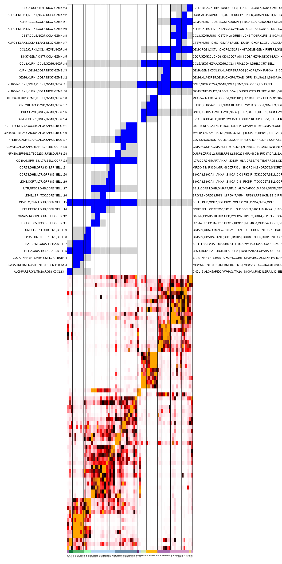

Clustered metacells confusion matrix

And the updated 2D projection would look like this:

#> agg_png 
#>       2

#> [1] TRUE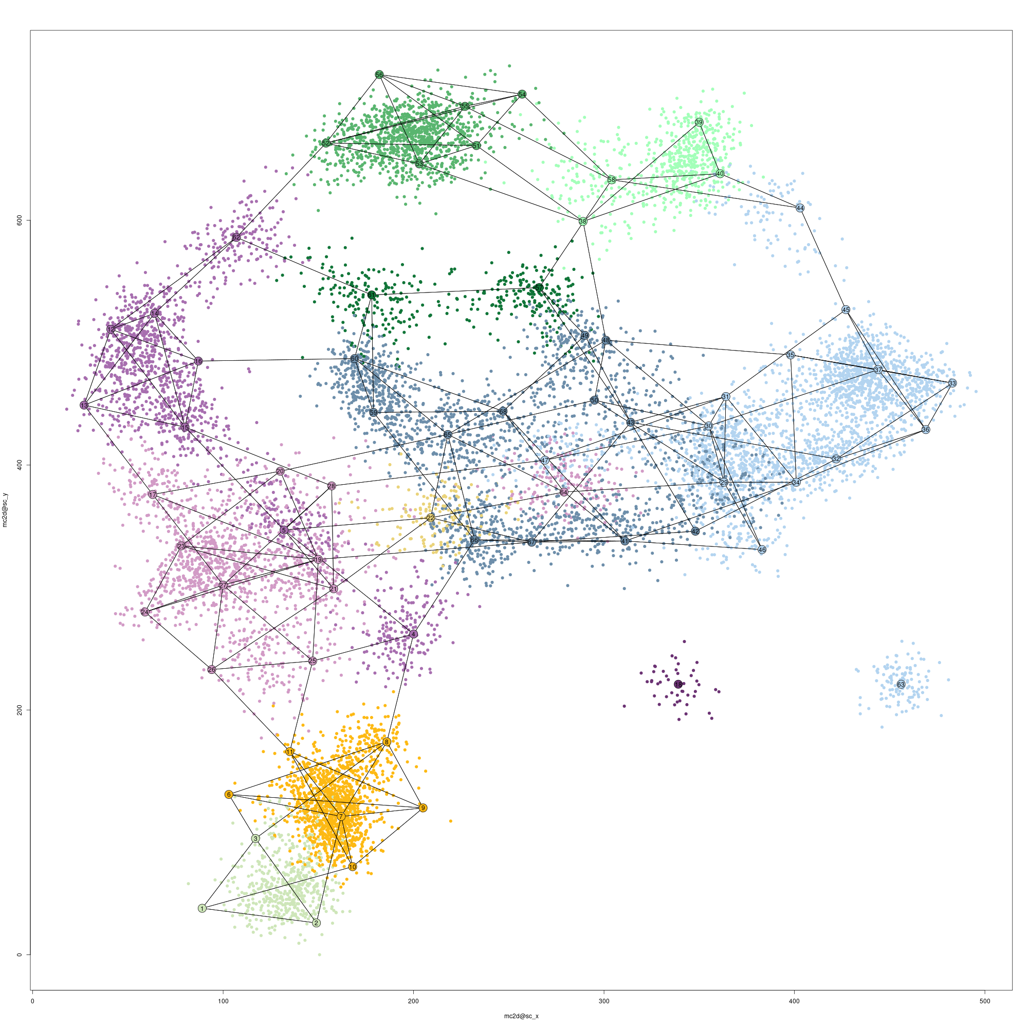

Single-cell and metacells 2D projection

Yaniv Lubling

2018-12-26

Introduction

Setting up

Initial exploration of the metacells

Metacells gene enrichment table

Manual annotation by thresholding gene enrichment

Systematic annotation of metacells