Running metacell analysis: guided tutorial on 8K PBMCs
A Tanay
2021-12-21
Source:vignettes/a-basic_pbmc8k.Rmd
a-basic_pbmc8k.RmdSetting up
In this note we demonstrate the basic MetaCell use on the small 8K PBMC data freely available from 10X Genomics. The guide includes import and manipulations of single cell RNA-seq count matrices, extraction of features genes, modeling cell-cell similarities and inference of a MetaCell model.
We start by loading the library:
To start using MetaCell, you first initialize a database. This is not much more than linking the package to directory that stores all your objects. In our case we will initialize the database to the testdb directory:
if(!dir.exists("testdb")) dir.create("testdb/")
scdb_init("testdb/", force_reinit=T)
#> initializing scdb to testdb/
force_reinit=T instruct the system to override existing database objects. This can be important if you are running in cycles and would like to update your objects. Otherwise, the database reuses loaded objects to save time on reading and initializing them from the disk.
Let's load a matrix to the system. We will import a 10x data set that is stored in the package datain directory, using a sparse matrix format generated by the 10x pipeline:
mcell_import_scmat_10x("test", base_dir="http://www.wisdom.weizmann.ac.il/~atanay/metac_data/pbmc_8k/")
#> remote mode
#> summing up total of 0 paralog genes into 0 unique genes
#> [1] TRUE
mat = scdb_mat("test")
print(dim(mat@mat))
#> [1] 29040  8364
The scdb_mat() command is returns a matrix object, which has one slot containing the count matrix - mat@mat, as well as additional features we will mention below.
Before starting to analyze the data, we link the package to a figure directory:
if(!dir.exists("figs")) dir.create("figs/")
scfigs_init("figs/")
MetaCell uses a standardized naming scheme for the figures, to make it easier to archive and link analysis figures to the database objects. In principle, figures in the figures directory are named after the object data type they refer to (for example, mat for matrices, mc for metacells, and more, see below). The figure name then includes also the object name they refer to, and a suffix describing the actual figure type.
Exploring and filtering the UMI matrix
To get a basic understanding of the new data, we will plot the distribution of UMI count per cell (the plot is thresholded at 800 UMIs by default):
mcell_plot_umis_per_cell("test")
#> [1] 300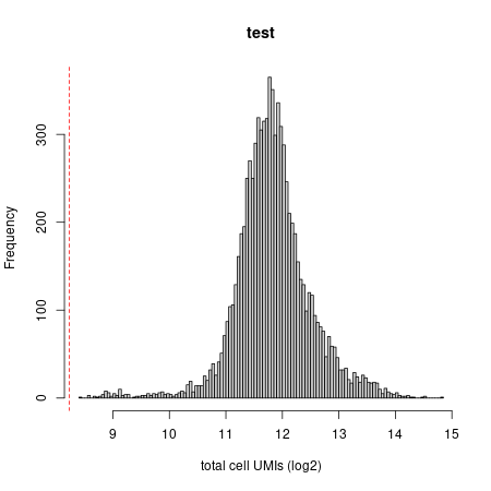
Umi distribution plot
We want to clean some known issues from the matrix before starting to work with it. We generate a list of mitochondrial genes that typically mark cells as being stressed or dying, as well as immunoglobulin genes that may represent strong clonal signatures in plasma cells, rather than cellular identity.
mat = scdb_mat("test")
nms = c(rownames(mat@mat), rownames(mat@ignore_gmat))
ig_genes = c(grep("^IGJ", nms, v=T),
                grep("^IGH",nms,v=T),
                grep("^IGK", nms, v=T),
                grep("^IGL", nms, v=T))

bad_genes = unique(c(grep("^MT-", nms, v=T), grep("^MTMR", nms, v=T), grep("^MTND", nms, v=T),"NEAT1","TMSB4X", "TMSB10", ig_genes))

bad_genes
#>   [1] "MT-ATP6"      "MT-ATP8"      "MT-CO1"       "MT-CO2"       "MT-CO3"
#>   [6] "MT-CYB"       "MT-ND1"       "MT-ND2"       "MT-ND3"       "MT-ND4"
#>  [11] "MT-ND4L"      "MT-ND5"       "MT-ND6"       "MT-RNR1"      "MT-RNR2"
#>  [16] "MT-TA"        "MT-TC"        "MT-TD"        "MT-TE"        "MT-TF"
#>  [21] "MT-TG"        "MT-TH"        "MT-TI"        "MT-TL1"       "MT-TL2"
#>  [26] "MT-TM"        "MT-TP"        "MT-TQ"        "MT-TS1"       "MT-TT"
#>  [31] "MT-TV"        "MT-TW"        "MT-TY"        "MTMR1"        "MTMR10"
#>  [36] "MTMR11"       "MTMR12"       "MTMR14"       "MTMR2"        "MTMR3"
#>  [41] "MTMR4"        "MTMR6"        "MTMR7"        "MTMR8"        "MTMR9"
#>  [46] "MTMR9LP"      "MTND1P11"     "MTND1P23"     "MTND1P32"     "MTND1P8"
#>  [51] "MTND2P12"     "MTND2P2"      "MTND2P28"     "MTND2P32"     "MTND2P40"
#>  [56] "MTND4LP30"    "MTND4P11"     "MTND4P12"     "MTND4P14"     "MTND4P32"
#>  [61] "MTND4P35"     "MTND4P9"      "MTND5P10"     "MTND5P11"     "MTND5P12"
#>  [66] "MTND5P14"     "MTND5P2"      "MTND5P26"     "MTND5P32"     "MTND5P33"
#>  [71] "MTND5P5"      "MTND6P21"     "MTND6P3"      "MTND6P4"      "MTND6P5"
#>  [76] "NEAT1"        "TMSB4X"       "TMSB10"       "IGHA1"        "IGHA2"
#>  [81] "IGHD"         "IGHD3-22"     "IGHD6-19"     "IGHD7-27"     "IGHE"
#>  [86] "IGHEP1"       "IGHEP2"       "IGHG1"        "IGHG2"        "IGHG3"
#>  [91] "IGHG4"        "IGHGP"        "IGHJ1"        "IGHJ2"        "IGHJ2P"
#>  [96] "IGHJ3P"       "IGHJ4"        "IGHJ5"        "IGHJ6"        "IGHM"
#> [101] "IGHMBP2"      "IGHV1-14"     "IGHV1-18"     "IGHV1-2"      "IGHV1-24"
#> [106] "IGHV1-3"      "IGHV1-46"     "IGHV1-67"     "IGHV1-69"     "IGHV1-69D"
#> [111] "IGHV2-26"     "IGHV2-5"      "IGHV2-70D"    "IGHV3-11"     "IGHV3-13"
#> [116] "IGHV3-15"     "IGHV3-21"     "IGHV3-23"     "IGHV3-30"     "IGHV3-33"
#> [121] "IGHV3-43"     "IGHV3-48"     "IGHV3-49"     "IGHV3-53"     "IGHV3-64D"
#> [126] "IGHV3-66"     "IGHV3-69-1"   "IGHV3-7"      "IGHV3-72"     "IGHV3-73"
#> [131] "IGHV3-74"     "IGHV3OR15-7"  "IGHV4-31"     "IGHV4-34"     "IGHV4-39"
#> [136] "IGHV4-4"      "IGHV4-59"     "IGHV4-61"     "IGHV5-10-1"   "IGHV5-51"
#> [141] "IGHV5-78"     "IGHV6-1"      "IGHVIII-76-1" "IGKC"         "IGKJ1"
#> [146] "IGKJ3"        "IGKJ4"        "IGKJ5"        "IGKV1-12"     "IGKV1-13"
#> [151] "IGKV1-16"     "IGKV1-17"     "IGKV1-27"     "IGKV1-39"     "IGKV1-5"
#> [156] "IGKV1-6"      "IGKV1-8"      "IGKV1-9"      "IGKV1D-13"    "IGKV1D-17"
#> [161] "IGKV1D-8"     "IGKV2-19"     "IGKV2-26"     "IGKV2-28"     "IGKV2-29"
#> [166] "IGKV2-30"     "IGKV2D-26"    "IGKV2D-28"    "IGKV2D-29"    "IGKV2D-40"
#> [171] "IGKV2OR2-1"   "IGKV3-11"     "IGKV3-15"     "IGKV3-20"     "IGKV3D-20"
#> [176] "IGKV4-1"      "IGKV5-2"      "IGLC2"        "IGLC3"        "IGLC4"
#> [181] "IGLC5"        "IGLC6"        "IGLC7"        "IGLJ2"        "IGLL1"
#> [186] "IGLL3P"       "IGLL5"        "IGLV1-40"     "IGLV1-41"     "IGLV1-44"
#> [191] "IGLV1-47"     "IGLV1-51"     "IGLV2-11"     "IGLV2-14"     "IGLV2-18"
#> [196] "IGLV2-23"     "IGLV2-5"      "IGLV2-8"      "IGLV3-1"      "IGLV3-10"
#> [201] "IGLV3-16"     "IGLV3-19"     "IGLV3-21"     "IGLV3-25"     "IGLV3-27"
#> [206] "IGLV3-9"      "IGLV4-69"     "IGLV5-37"     "IGLV5-45"     "IGLV6-57"
#> [211] "IGLV7-43"     "IGLV7-46"     "IGLV8-61"     "IGLVI-20"
We will next ask the package to ignore the above genes:
mcell_mat_ignore_genes(new_mat_id="test", mat_id="test", bad_genes, reverse=F) Ignored genes are kept in the matrix for reference, but all downstream analysis will disregard them. This means that the number of UMIs from these genes cannot be used to distinguish between cells.
In the current example we will also eliminate cells with less than 800 UMIs (threshold can be set based on examination of the UMI count distribution):
mcell_mat_ignore_small_cells("test", "test", 800)Note that filtering decisions can be iteratively modified given results of the downstream analysis.
Selecting feature genes
We move on to computing statistics on the distributions of each gene in the data, which are going to be our main tool for selecting feature genes for MetaCell analysis:
mcell_add_gene_stat(gstat_id="test", mat_id="test", force=T)
#> Calculating gene statistics...
#> will downsamp
#> done downsamp
#> will gen mat_n
#> done gen mat_n
#> done computing basic gstat, will compute trends
#> ..done
This generates a new object of type gstat under the name "test", by analyzing the count matrix with id "test". We can explore interesting genes and their distributions, or move directly to select a gene set for downstream analysis. For now, let's to the latter.
We create a new object of type gset (gene set), to which all genes whose scaled variance (variance divided by mean) exceeds a given threshold are added:
mcell_gset_filter_varmean(gset_id="test_feats", gstat_id="test", T_vm=0.08, force_new=T)
mcell_gset_filter_cov(gset_id = "test_feats", gstat_id="test", T_tot=100, T_top3=2)
The first command creates a new gene set with all genes for which the scaled variance is 0.08 and higher. The second command restrict this gene set to genes with at least 100 UMIs across the entire dataset, and also requires selected genes to have at least three cells for more than 2 UMIs were recorded.
We can refine our parameters by plotting all genes and our selected gene set given the mean and variance statistics:
mcell_plot_gstats(gstat_id="test", gset_id="test_feats")
#> agg_png
#>       2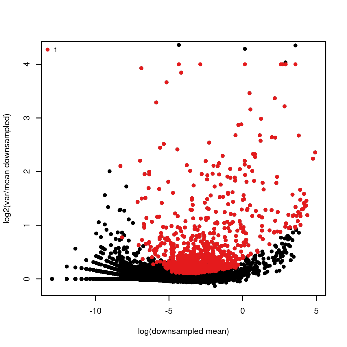
var mean plot
Building the balanced cell graph
Assuming we are happy with the selected genes (some strategies for studying them will be discussed in another vignette), we will move forward to create a similarity graph (cgraph), using a construction called balanced K-nn graph:
mcell_add_cgraph_from_mat_bknn(mat_id="test",
                gset_id = "test_feats",
                graph_id="test_graph",
                K=100,
                dsamp=T)
#> will downsample the matrix, N= 1877
#> will build balanced knn graph on 8276 cells and 919 genes, this can be a bit heavy for >20,000 cells
#> sim graph is missing 34 nodes, out of 8276
This adds to the database a new cgraph object named test_graph. The K=100 parameter is important, as it affects the size distribution of the derived metacells. Note that constructing the graph can become computationally intensive if going beyond 20-30,000 cells. The system is currently limited by memory, and we have generated a graph on 160,000 cells on machines with 0.5TB RAM. For more modest data sets (e.g. few 10x lanes or MARS-seq experiments), things will run very quickly.
Resampling and generating the co-clustering graph
The next step will use the cgraph to sample five hundred metacell partitions, each covering 75% of the cells and organizing them in dense subgraphs:
mcell_coclust_from_graph_resamp(
                coc_id="test_coc500",
                graph_id="test_graph",
                min_mc_size=20,
                p_resamp=0.75, n_resamp=500)
#> running bootstrap to generate cocluster
#> done resampling
The metacell size distribution of the resampled partitions will be largely determined by the K parameter used for computing the cgraph. The resampling process may take a while if the graphs are very large. You can modify n_resamp to generate fewer resamples.
The resampling procedure creates a new coclust object in the database named test_coc500, and stores the number of times each pair of cells ended up being part of the same metacell. The co-clustering statistics are used to generate a new similarity graph, based on which accurate calling of the final set of metacells is done:
mcell_mc_from_coclust_balanced(
                coc_id="test_coc500",
                mat_id= "test",
                mc_id= "test_mc",
                K=30, min_mc_size=30, alpha=2)
#> filtered 4328387 left with 717178 based on co-cluster imbalance
#> building metacell object, #mc 75
#> add batch counts
#> compute footprints
#> compute absolute ps
#> compute coverage ps
#> reordering metacells by hclust and most variable two markers
#> reorder on CD74 vs JUNB
We created a metacell object test_mc based on analysis of the co-clustering graph. The parameter K determines the number of neighbors we wish to minimally associate with each cell. Prior to partitioning the co-cluster graph is filtered to eliminate highly unbalanced edges, with smaller alpha resulting in harsher filtering.
Removing outlier cells
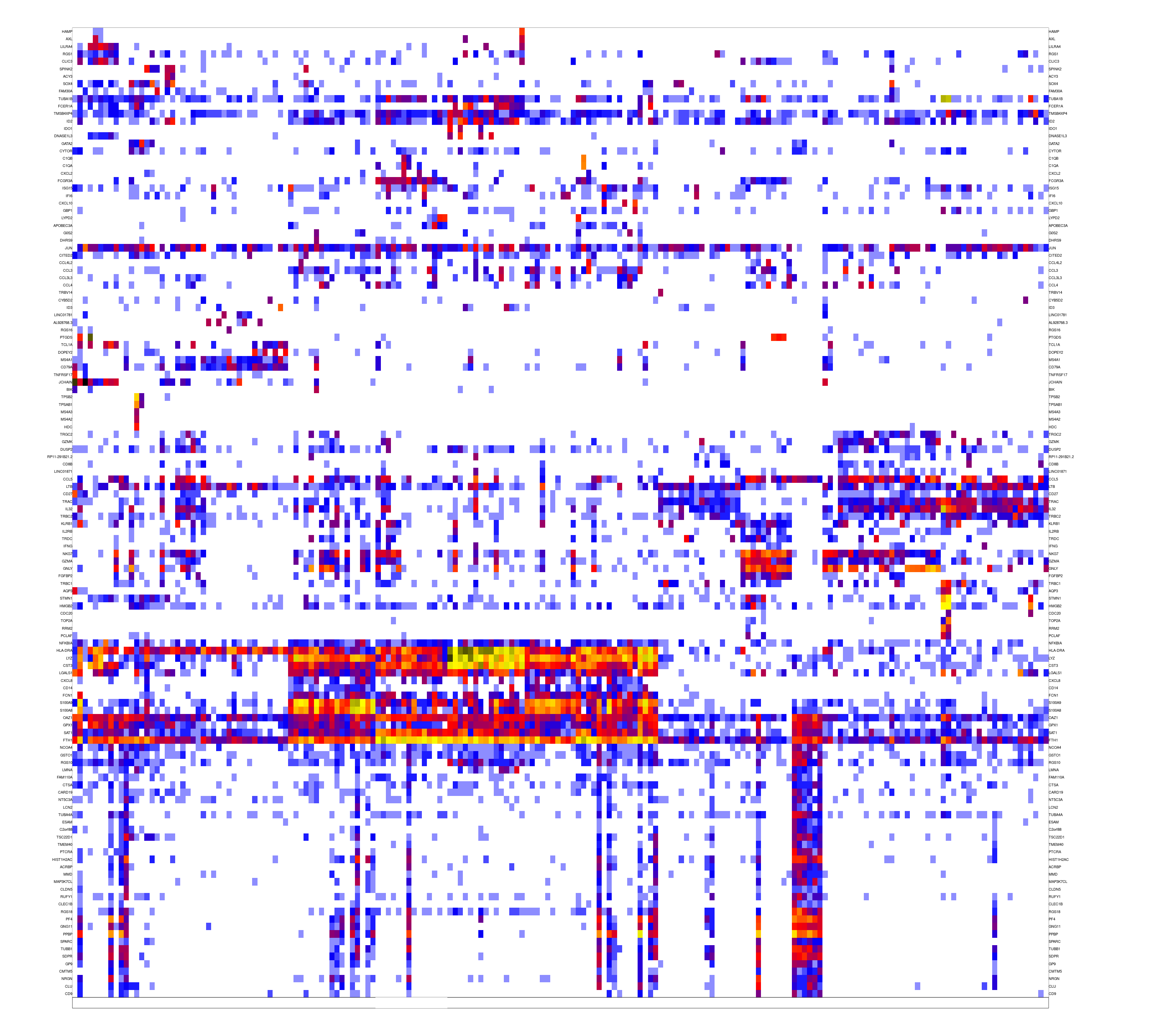
We now have a preliminary metacell object. It is a good practice to make sure all metacells within it are homogeneous. This is done by the outlier scan procedure, which splits metacells whose underlying similarity structure supports the existence of multiple sub-clusters, and removes outlier cells that strongly deviate from their metacell's expression profile.
mcell_plot_outlier_heatmap(mc_id="test_mc", mat_id = "test", T_lfc=3)
#> agg_png
#>       2
mcell_mc_split_filt(new_mc_id="test_mc_f",
            mc_id="test_mc",
            mat_id="test",
            T_lfc=3, plot_mats=F)
#> starting split outliers
#> add batch counts
#> compute footprints
#> compute absolute ps
#> compute coverage ps
The first command generates a heat map summarizing the detected outlier behaviors. This is possible only for data sets of modest size.
outliers fig
Selecting markers and coloring metacells
The filtered metacell object test_mc_f can now be visualized. In order to do this effectively, we usually go through one or two iterations of selecting informative marker genes. The package can select markers for you automatically - by simply looking for genes that are strongly enriched in any of the metacells:
mcell_gset_from_mc_markers(gset_id="test_markers", mc_id="test_mc_f")It is however very useful to analyze metacell models in depth, and select genes with known or hypothesized biological significance. We will assign each of these genes with a color, fold change threshold and priority, using a table that look like this:
| group | gene | color | priority | T_fold |
|---|---|---|---|---|
| NK | CLIC3 | brown | 4 | 8 |
| NK_KLRF1 | KLRF1 | chocolate3 | 8 | 3 |
| CD8 | CD8B | yellow | 5 | 2 |
| T+GMZK | GZMK | sienna1 | 5 | 4 |
| Mk+COMP | C1QA | darkolivegreen | 5 | 2 |
| S100A9 | S100A9 | darkseagreen3 | 5 | 20 |
| LYZ | LYZ | chartreuse | 4 | 8 |
| B | CD79B | lightblue | 4 | 4 |
| MZB1 | MZB1 | cyan | 5 | 4 |
| IRF8 | IRF8 | cyan2 | 5 | 4 |
| IL7R | IL7R | navajowhite2 | 3 | 2 |
| Treg | FOXP3 | magenta | 5 | 1.5 |
| CD3 | CD3G | lemonchiffon | 1 | 0.7 |
Applying this table to color metacells is done using the command mc_colorize as shown below. Note that there are more sophisticated ways to color/annotate metacells, and that the model's understanding and annotation can often greatly benefit from looking at gene distributions and reading literature about possible functions and regulatory mechanisms.
marks_colors = read.table(system.file("extdata", "pbmc_mc_colorize.txt", package="metacell"), sep="\t", h=T, stringsAsFactors=F)
mc_colorize("test_mc_f", marker_colors=marks_colors)
We are now equipped with some basic coloring of metacells, which can also be accessed directly:
Creating a heatmap of genes and metacells
We can use the colors to produce a labeled heat map, showing selected genes and their distributions over metacells, with the colored annotation shown at the bottom:
mcell_mc_plot_marks(mc_id="test_mc_f", gset_id="test_markers", mat_id="test")
#> setting fig h to 1000 md levels 0 num of marks 48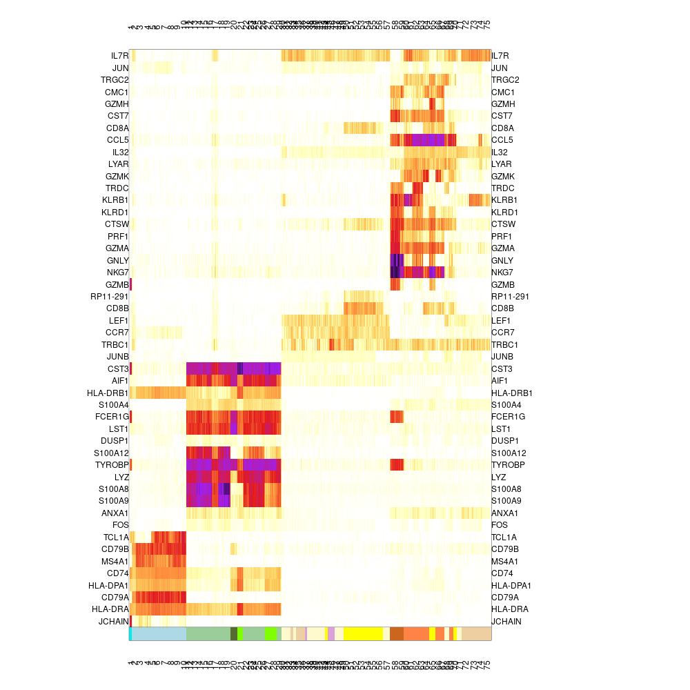
heatmap_marks
Note that the values plotted are color coded log2(fold enrichment) value of the metacell over the median of all other metacells. It can be useful to explore these values directly - e.g.:
Projecting metacells and cells in 2D
Heat maps are useful but sometimes hard to interprets, and so we may want to visualize the similarity structure among metacells (or among cells within metacells). To this end we construct a 2D projection of the metacells, and use it to plot the metacells and key similarities between them (shown as connecting edges), as well as the cells. This plot will use the same metacell coloring we established before (and in case we improve the coloring based on additional analysis, the plot can be regenerated):
mcell_mc2d_force_knn(mc2d_id="test_2dproj",mc_id="test_mc_f", graph_id="test_graph")
#> comp mc graph using the graph test_graph and K 20
#> Missing coordinates in some cells that are not ourliers or ignored - check this out! (total 1 cells are missing, maybe you used the wrong graph object? first nodes CCCTCCTAGTCGCCGT
tgconfig::set_param("mcell_mc2d_height",1000, "metacell")
tgconfig::set_param("mcell_mc2d_width",1000, "metacell")
mcell_mc2d_plot(mc2d_id="test_2dproj")
#> agg_png
#>       2
Note that we changed the metacell parameters "mcell_mc2d_height/width" to get a reasonably-sized figure. There are many additional parameters that can be tuned in MetaCell, and more of those meant for routine tuning will be discussed in other vignettes. We obtain the following figure:
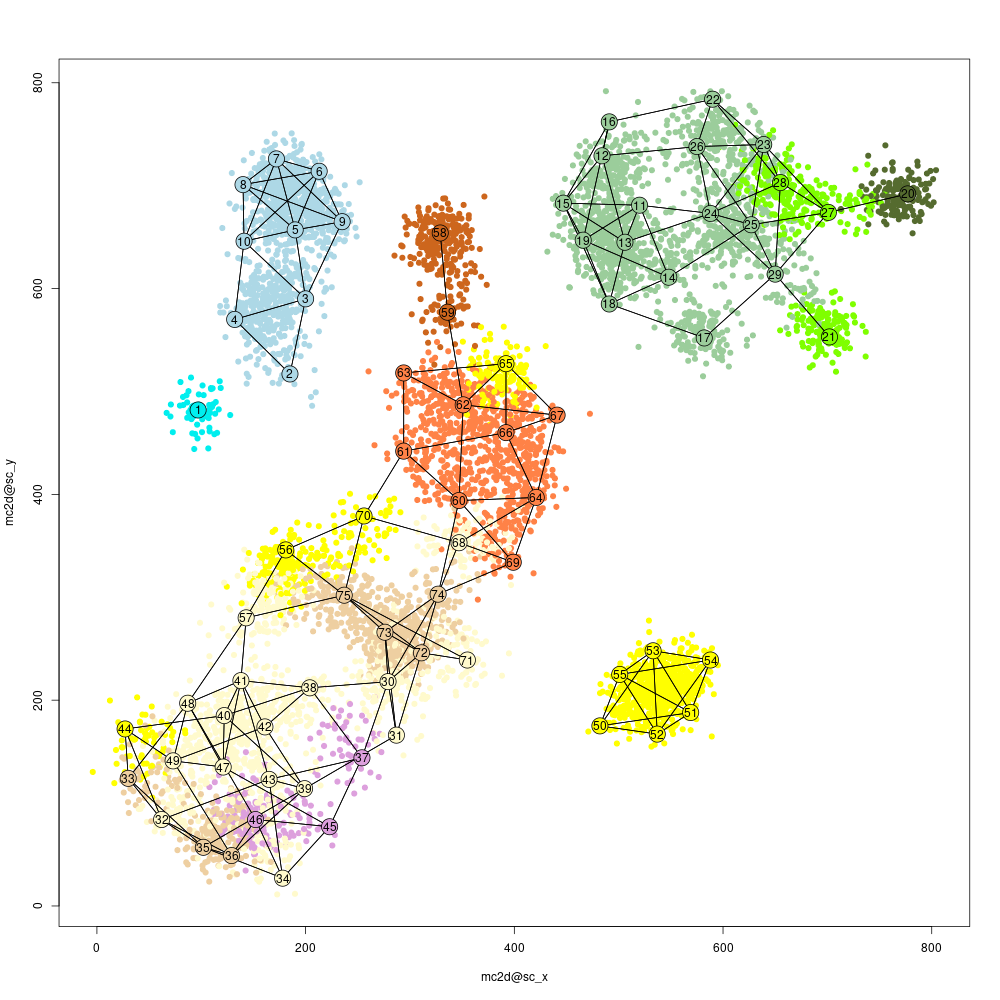
proj2d mean plot
Visualizing the MC confusion matrix
While 2D projections are popular and intuitive (albeit sometimes misleading) ways to visualize scRNA-seq results, we can also summarize the similarity structure among metacells using a "confusion matrix" which encodes the pairwise similarities between all metacells. This matrix may capture hierarchical structures or other complex organizations among metacells.
We first create a hierarchical clustering of metacells, based on the number of similarity relations between their cells:
mc_hc = mcell_mc_hclust_confu(mc_id="test_mc_f",
                                            graph_id="test_graph")
Next, we generate clusters of metacells based on this hierarchy, and visualize the confusion matrix and these clusters. The confusion matrix is shown at the bottom, and the top panel encodes the cluster hierarchy (subtrees in blue, sibling subtrees in gray):
mc_sup = mcell_mc_hierarchy(mc_id="test_mc_f",
                                                    mc_hc=mc_hc, T_gap=0.04)
mcell_mc_plot_hierarchy(mc_id="test_mc_f",
                   graph_id="test_graph",
                    mc_order=mc_hc$order,
                    sup_mc = mc_sup,
                    width=2800, heigh=2000, min_nmc=2)
#> agg_png
#>       2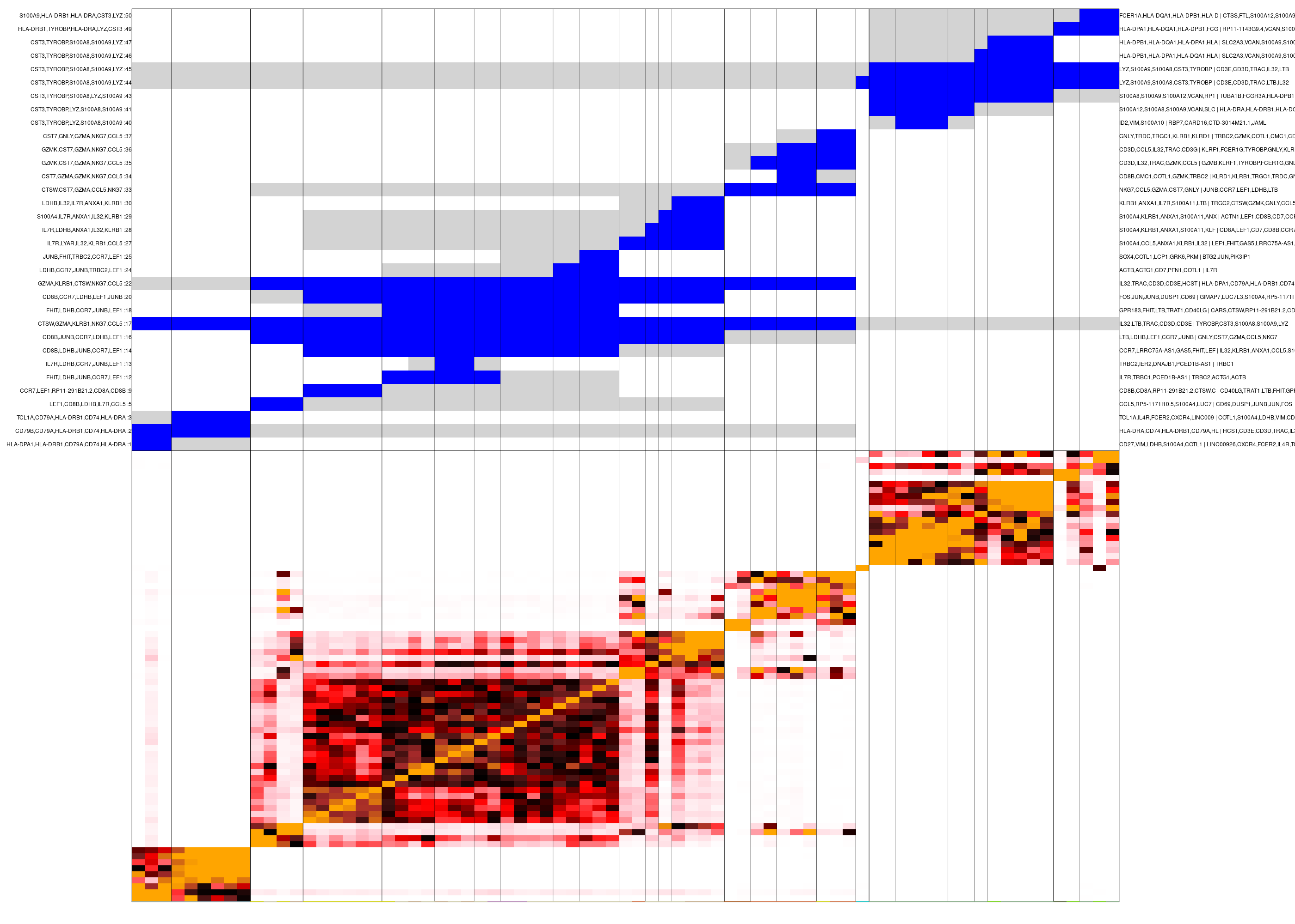
confusion matrix